Practical Robotics and Computer Vision (BPC-PRP)
This is a complete lab documentations for the BPC-PRP course at FEEC, Brno University of Technology.
In this course studets are aiming to program robot to fealize maze escape task.
Authors
- Ing. Adam Ligocki, Ph.D.
- Ing. Petr Šopák
- Ing Jakub Minařík
Acknowledgments
This work was created with the support of project RP182401001 under the PPSŘ 2025 program.
Lectures
Overview
Week 1 - Course Introduction
- Course introductions
- Instructors
- Organization
- Assessment overview (tests and final exam)
Responsible: Ing. Adam Ligocki, Ph.D.
Week 2 - Linux OS, C++, CMake, Unit Tests
- Linux OS overview, command line interface, basic programs
- Compiling a simple program using GCC
- Simple CMake project
- Unit tests
Responsible: Ing. Jakub Minařík
Week 3 - Git
- Git basics
- Online Git services
- Code quality (formatting, static analysis, ...)
Responsible: Ing. Adam Ligocki, Ph.D.
Week 4 - ROS2 Basics
- Elementary concepts of ROS2
- RViz
Responsible: Ing. Jakub Minařík
Week 5 - Kinematics & Odometry
- Differential chassis
- Wheel odometry
Responsible: Ing. Adam Ligocki, Ph.D.
Week 6 - Line Detection & Estimation
- Line sensor
- Differential sensor
- Line distance estimation
Responsible: Ing. Petr Šopák
Week 7 - Control Loop
- Line following principles
- Bang-bang controller
- P(I)D controller
Responsible: Ing. Adam Ligocki, Ph.D.
Week 8 - ROS2 Advanced
- DDS, node discovery
- launch system
- Visualization (markers, TFs, URDF, ...)
- Gazebo Responsible: Ing. Jakub Minařík
Week 9 - Robot Sensors & Architecture
- Understanding the range of robot sensors
- Deep dive into robot architecture
Responsible: Ing. Adam Ligocki, Ph.D.
Week 10 - Computer Vision 1
- CV overview
- Basic algorithms
- Image sensors
- Raspberry Pi & camera
Responsible: Ing. Petr Šopák
Week 11 - Computer Vision 2
- OpenCV usage
- ArUco detection
Responsible: Ing. Petr Šopák
Week 12 - Substitute Lecture
- To be announced (TBA)
Responsible: Ing. Adam Ligocki, Ph.D.
Exam Period - Final Exam
- Practical test (Maze escape task)
Laboratories
Overview
Lab 1 - Development Environment & First C++ Program
- Introduction to laboratory
- Linux Command Line Interface (CLI)
- C++ Review
- CLI compilation
- CLion and ROS 2 introduction
Responsible: Ing. Petr Šopák
Lab 2 - Project Workflow: Git, CMake & Team Project
- Git Basics and workflow
- Simple CMake project
- Unit tests
- Online repository
- Course project template
Responsible: Ing. Petr Šopák
Lab 3 - Data Capture & Visualization (ROS)
- ROS 2 in CLI
- Simple Node, Publisher, Subscriber
- RViz, Data Visualization
Responsible: Ing. Petr Šopák
Lab 4 - Motor, Kinematics & Gamepad
- Motor Control
- Forward and Inverse Kinematics
- Gamepad
Responsible: Ing. Jakub Minařík
Lab 5 - Line Estimation
- Line Sensor Usage
- Line Position Estimation
- Line Sensor Calibration
Responsible: Ing. Adam Ligocki, Ph.D.
Lab 6 - Line Following & PID
- Line Following Control Loop Implementation
Responsible: Ing. Petr Šopák
Lab 7 - Midterm Test (Line Following)
- Good Luck
Responsible: Ing. Adam Ligocki, Ph.D.
Lab 8 - LiDAR
- Understanding LiDAR data
- LiDAR Data Filtration
- Corridor Following Algorithm
Responsible: Ing. Petr Šopák
Lab 9 - Inertial Measurement Unit (IMU)
- Understanding IMU Data
- Orientation Estimation Using IMU
Responsible: Ing. Petr Šopák
Lab 10 - Camera Data Processing
- Understanding Camera Data
- ArUco Detection Library
Responsible: Ing. Petr Šopák
Lab 11 - Individual work
- Individual work
- Consultation
Responsible: Ing. Petr Šopák
Lab 12 - Midterm Test (Corridor Following)
- Good Luck!
Responsible: Ing. Adam Ligocki, Ph.D.
Final Exam - Maze Escape
- Good Luck!
Responsible: Ing. Adam Ligocki, Ph.D.
Lab 1 - Development Environment & First C++ Program
Responsible: Ing. Petr Šopák
This laboratory introduces the basic development environment used throughout the BPC-PRP course.
The goal is to get familiar with Linux, command-line tools, and to compile and run a simple C++ program.
By the end of this lab, you should be able to:
- navigate the Linux file system using the CLI,
- create and edit source files,
- compile and run a basic C++ program,
- understand the role of an IDE and ROS 2 in this course.
Linux & Command Line Basics (≈ 60 min)
Installation (optional)
To install Linux, please follow the Linux chapter.
Exercise
- Explore the system GUI.
- Open a terminal and navigate the file system.
- Practice basic CLI commands (see the Linux chapter):
- Check the current directory:
pwd - Create a directory:
mkdir <dir> - Enter a directory:
cd <dir> - Create a file:
touch <file> - List directory contents:
ls -la - Rename or move a file:
mv <old> <new> - Copy a file:
cp <src> <dst> - Remove a file:
rm <file> - Create/remove a directory:
mkdir <dir>,rm -r <dir>
- Check the current directory:
- Try a text editor:
nanoorvim
I installed vim and accidentally opened it. What now?
You can exit Vim with: press Esc, then hold Shift and press Z twice (Shift+Z+Z).More Info: https://www.vim.org/docs.php
More details about Linux will be introduced during the course.
First C++ Program – CLI Compilation (≈ 60 min)
Create a new project folder in your home directory and enter it.
Create a file main.cpp with the following content:
#include <iostream>

#define A 5

int sum(int a, int b) {
    return a + b;
}

int main() {
    std::cout << "My first C++ program" << std::endl;
    int b = 10;
    std::cout << "Sum result: " << sum(A, b) << std::endl;
    return 0;
}
Compile the program using g++ (GCC C++ compiler):
g++ -o my_program main.cpp
Run the compiled binary:
./my_program
There are other alternatives, like Clang, LLVM, and many others.
TASK 1
- In your project folder, create an
includefolder. - In the
includefolder, create alib.hppfile and write a simple function in it. - Use the function from
lib.hppinmain.cpp. - Compile and run the program (tip: use
-I <folder>with g++ to specify the header search path).
TASK 2
- In the project folder, create
lib.cpp. - Move the function implementation from
lib.hpptolib.cpp; keep the function declaration inlib.hpp. - Compile and run the program (tip: you have to compile both
main.cppandlib.cpp). - Helper:
g++ -o <output_binary> <source_1.cpp source_2.cpp ...> -I <folder_with_headers> - Discuss the difference between preprocessing, compiling, and linking.
IDE Overview – CLion (≈ 15 min)
Installation
Install CLion using the Snap package manager:
sudo snap install --classic clion
Alternatively, download CLion from the official website and get familiar with it (see CLion IDE). By registering with your school email, you can obtain a free student license.
To learn how to control CLion, please take a look at the tutorial or the official docs.
TASK 3
- Learn how to control CLion
- Open the previously created C++ program (main.cpp) in CLion.
- Build and run the program using the IDE controls.
ROS 2 – Course Context (≈ 15 min)
ROS 2 (Robot Operating System 2) is a framework for building robotic systems. In this course, ROS 2 will be used later for:
- communication between software components,
- visualization (RViz, rqt),
simulation (Gazebo).
For installation and basic commands, see the ROS 2 chapter: ROS 2.
Lab 2 - Project Workflow: Git, CMake & Team Project
Responsible: Ing. Petr Šopák
This laboratory introduces the software development workflow used in the rest of the BPC-PRP course.
You will learn how to manage source code using Git, how C++ projects are structured, and how to build them using CMake.
The project created in this lab will serve as a base project for subsequent laboratories.
By the end of this lab, you should be able to:
- use Git for version control and teamwork,
- clone, commit, push, pull, and resolve merge conflicts,
- understand the structure of a C++ project,
- build a project using CMake,
- work with a shared repository in a team.
Git Basics & Team Workflow (≈ 75 min)
Before starting, read the Git tutorial.
Sign-up
Register on one of the following Git services:
This server will serve as your "origin" (remote repository) for the rest of the BPC-PRP course.
The instructors will have access to all your repositories, including their history, and can monitor your progress, including who, when, and how frequently commits were made.
Create a repository on the server to maintain your code throughout the course.
Cloning the Repository
HTTPS - GitHub Token
When cloning a repository via HTTPS, you cannot push changes using your username and password. Instead, you must use a generated GitHub token.
To generate a token, go to Profile picture (top-right corner) > Settings > Developer Settings > Personal Access Tokens > Tokens (classic) or click here. Your generated token will be shown only once, after which you can use it as a password when pushing changes via HTTPS until the token expires.
SSH - Setting a Different Key
You can generate an SSH key using the ssh-keygen command. It will prompt you for the file location/name and then for a passphrase. For lab use, set a passphrase. The default location is ~/.ssh.
When cloning a repository via SSH in the lab, you may encounter a problem with Git using the wrong SSH key.
You'll need to configure Git to use your generated key:
git config core.sshCommand "ssh -i ~/.ssh/<your_key>"
In this command, <your_key> refers to the private part of your generated key.
On GitHub, you can add the public part of your key to either a specific repository or your entire account.
-
To add a key to a project (repository level):
Go to Project > Settings > Deploy keys > Add deploy key, then check Allow write access if needed. -
To add a key to your GitHub account (global access):
Go to Profile picture (top-right corner) > Settings > SSH and GPG keys > New SSH key.
Team Task
As a team, complete the following steps:
- One team member creates a repository on the server.
- All team members clone the repository to their local machines.
- One team member creates a "Hello, World!" program locally, commits it, and pushes it to the origin.
- The rest of the team pulls the changes to their local repositories.
- Two team members intentionally create a conflict by modifying the same line of code simultaneously and attempting to push their changes to the server. The second member to push will receive an error from Git indicating a conflict.
- The team member who encounters the conflict resolves it and pushes the corrected version to the origin.
- All team members pull the updated version of the repository. Each member then creates their own
.hfile containing a function that prints their name. Everyone pushes their changes to the server. - One team member pulls the newly created
.hfiles and modifies the "Hello, World!" program to use all the newly created code. The changes are then pushed to the origin. - All team members pull the latest state of the repository.
Project Structure & CMake (≈ 60 min)
Before continuing, get familiar with CMake.
Now let's create a similar project from last lab, but using CMake.
- Determine your current location in the file system.
- Switch to your home directory.
- Create a new project folder.
- Inside this folder, create several subdirectories so that the structure looks like this (use the tree command to verify):
/MyProject
 |--build
 |--include
 | \--MyProject
 \--src
- Using any text editor (like
nanoorvim), create the following files in the project root:main.cpp,lib.cpp,lib.hpp, andCMakeLists.txt. - Move (do not copy) the
main.cppandlib.cppfiles into thesrcsubdirectory. - Move the
lib.hppfile into theinclude/MyProjectsubdirectory. - Move the
CMakeLists.txtfile into the root of the project folder.
Now your project should look like this:
/MyProject
 |--build
 |--CMakeLists.txt
 |--include
 | \--MyProject
 |   \--lib.hpp
 \--src
   |--lib.cpp
   \--main.cpp
- Using a text editor, fill the
main.cpp,lib.cpp, andlib.hppfiles with the required code. - Using a text editor, fill the
CMakeLists.txtfile.
cmake_minimum_required(VERSION 3.10)
project(MyProject)
set(CMAKE_CXX_STANDARD 17)
include_directories(include/)
add_executable(my_program src/main.cpp src/lib.cpp)
Now compile the project. From the project folder, run:
cd my_project_dir  # go to your project directory
mkdir -p build     # create build folder
cd build           # enter the build folder
cmake ..           # configure; looks for CMakeLists.txt one level up
make               # build program
./my_program       # run program
Optional: Try to compile the program manually.
g++ <source1 source2 source3 ...> -I <include_directory> -o <output_binary>
- Delete project folder
BONUS TASK
Create the same project using the CLion IDE.
To learn how to control CLion, please take a look at the tutorial or the official docs.
Unit Tests, GTest (30 min)
Unit tests are an effective way to develop software. Often called test‑driven development, the idea is: define the required functionality, write tests that cover the requirements, and then implement the code. When tests pass, the requirements are met.
On larger projects with many contributors and frequent changes, unit tests help catch regressions early. This supports Continuous Integration (CI).
There are many testing frameworks. In this course we will use GoogleTest (GTest), a common and well‑supported choice for C++.
GTest Installation
If there is no GTest installed on the system follow these instructions.
# install necessary packages
sudo apt update
sudo apt install cmake build-essential libgtest-dev

# compile gtest
cd /usr/src/gtest
sudo cmake .
sudo make

# install libs into system
sudo cp lib/*.a /usr/lib
Verify the libraries are in the system:
ls /usr/lib | grep gtest

# you should see:
# libgtest.a
# libgtest_main.a
Adding Unit Test to Project
In your project directory add the test folder.
/MyProject
 |--include
 |--src
 \--test
Add the add_subdirectory(test) line at the end of CMakeLists.txt file.
Create CMakeLists.txt file in the test folder.
cmake_minimum_required(VERSION 3.10)

find_package(GTest REQUIRED)
include(GoogleTest)
enable_testing()

add_executable(my_test my_test.cpp)
target_link_libraries(my_test GTest::GTest GTest::Main)
gtest_discover_tests(my_test)
Create my_test.cpp file.
#include <gtest/gtest.h>

// Simple addition function for demonstration.
float add(float a, float b) {
    return a + b;
}

TEST(AdditionTest, AddsPositiveNumbers) {
    EXPECT_FLOAT_EQ(add(5.0f, 10.0f), 15.0f);
    EXPECT_FLOAT_EQ(add(0.0f, 0.0f), 0.0f);
}

TEST(AdditionTest, AddsEqualNumbers) {
    EXPECT_FLOAT_EQ(add(10.0f, 10.0f), 20.0f);
}

int main(int argc, char** argv) {
    testing::InitGoogleTest(&argc, argv);
    return RUN_ALL_TESTS();
}
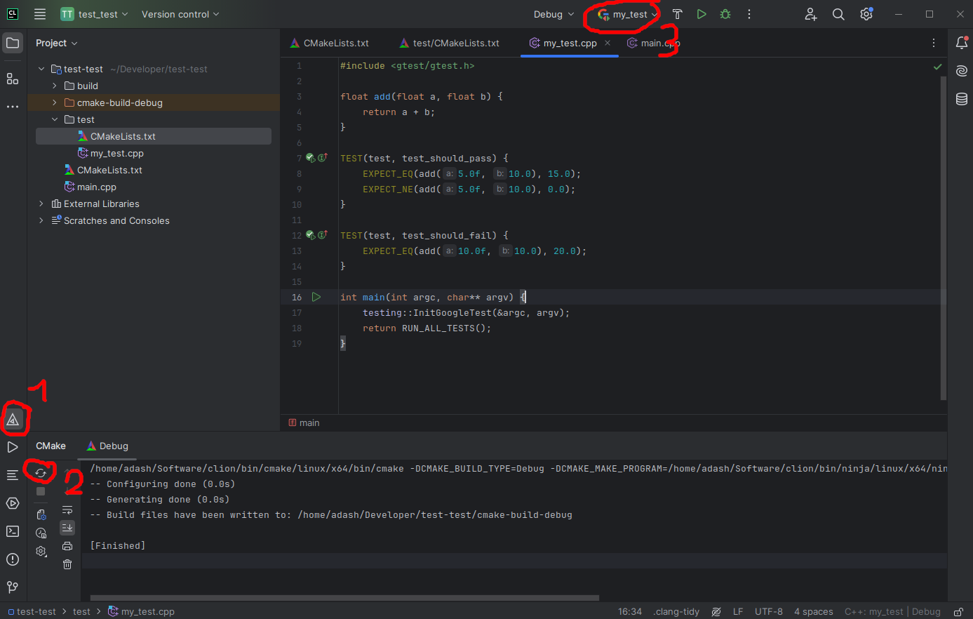
In CLion, open the bottom console and run:
mkdir build && cd build
cmake ..
make
cd test
ctest
You should see the test output.
You can also run tests directly in CLion by reloading CMake; the test target will appear as an executable at the top of the window.
C++ Training (2h)
Take a look at the basic C++ tutorial and the more advanced multithreading tutorial.
Lab 3 - Data Capture & Visualization (ROS)
Responsible: Ing. Petr Šopák
Learning objectives
1) Fundamentals of ROS 2
- Setting Up a ROS 2 workspace (optional)
- Creating a custom ROS 2 node - implementing a basic publisher & subscriber
- Exploring essential ROS 2 CLI commands
- Utilizing visualization tools -
rqt_plotandrqt_graph
2) Implementing Basic Behavior for BPC-PRP robots
- Establishing connection to the robots
- Implementing IO node - Reading button inputs and controlling LEDs
BONUS: Advanced Visualizations
- Using RViz2 for graphical representation
- Creating basic graphical objects and defining their behavior
If you are using your own notebook, make sure to configure everything necessary in the Ubuntu environment! Refer to Ubuntu Environment Chapter for details.
Fundamentals of ROS 2 (Approx. 1 Hour)
Setting Up a ROS Workspace (5 min) - optional
Last week, you cloned a basic template that we will gradually extend with additional functionalities. The first step is to establish communication between the existing project and ROS 2.
There are many ways to set up a ROS project, but typically, a ROS workspace is created, which is a structured directory for managing multiple packages. However, for this course, we do not need a full ROS workspace, as we will be working with only one package. Let’s review the commands from Lab 1. Using the CLI, create a workspace folder structured as follows:
mkdir -p ~/ros_w/src
cd ~/ros_w
Next, copy the folders from previous labs into the src directory or re-clone the repository from Git (Lab 3). You can rename the template to something like "ros_package", but this is optional.
Finally, you need to compile the package and set up the environment:
colcon build
source install/setup.bash
Recap Notes: What is a ROS Workspace?
A ROS workspace is a structured environment for developing and managing multiple ROS packages. In this case, we created a workspace named ros_w (you can choose any name, but this follows common convention).
A ROS workspace allows for unified compilation and management of multiple packages. Each ROS package is a CMake project stored in the
srcfolder. Packages contain:
- Implementations of nodes (executable programs running in ROS),
- Definitions of messages (custom data structures used for communication),
- Configuration files,
- Other resources required for running ROS functionalities.
After (or before) setting up the workspace, always remember to source your environment before using ROS:
source ~/ros_w/install/setup.bashor add sourcing to your shell startup script
echo "source /opt/ros/<distro>/setup.bash" >> ~/.bashrc
Creating a custom node (55 min)
In this section, we will create a ROS 2 node that will publish and receive data (info). We will then visualize the data accordingly.
Required Tools:
Instructions:
-
Open a terminal and set the ROS_DOMAIN_ID to match the ID on your computer’s case:
export ROS_DOMAIN_ID=<robot_ID>This change is temporary and applies only to the current terminal session. If you want to make it permanent, you need to update your configuration file:
echo "export ROS_DOMAIN_ID=<robot_ID>" >> ~/.bashrc
source ~/.bashrc
Check the contents of
~/.bashrc. The file runs at the start of each new Bash session and sets up your environment.cat ~/.bashrcTo verify the domain ID, use:
echo $ROS_DOMAIN_IDIf there are any issues with the .bashrc file, please let me know.
-
Open your CMake project in CLion or another Editor/IDE
-
Ensure that the IDE is launched from a terminal where the ROS environment is sourced
source /opt/ros/<distro>/setup.bash # We are using the Humble distribution
- Write the following code in
main.cpp:
#include <rclcpp/rclcpp.hpp>
#include "RosExampleClass.h"

int main(int argc, char* argv[]) {
    rclcpp::init(argc, argv);

    // Create an executor (for handling multiple nodes)
    auto executor = std::make_shared<rclcpp::executors::MultiThreadedExecutor>();

    // Create multiple nodes
    auto node1 = std::make_shared<rclcpp::Node>("node1");
    auto node2 = std::make_shared<rclcpp::Node>("node2");

    // Create instances of RosExampleClass using the existing nodes
    auto example_class1 = std::make_shared<RosExampleClass>(node1, "topic1", 1.0);
    auto example_class2 = std::make_shared<RosExampleClass>(node2, "topic2", 2.0);

    // Add nodes to the executor
    executor->add_node(node1);
    executor->add_node(node2);

    // Run the executor (handles callbacks for both nodes)
    executor->spin();

    // Shutdown ROS 2
    rclcpp::shutdown();
    return 0;
}
- Create a header file in the
includedirectory to ensure the code runs properly. - Add the following code to the header file:
#pragma once

#include <iostream>
#include <string>
#include <rclcpp/rclcpp.hpp>
#include <std_msgs/msg/float32.hpp>
#include <chrono>

class RosExampleClass {
public:
    // Constructor takes a shared_ptr to an existing node instead of creating one.
    RosExampleClass(const rclcpp::Node::SharedPtr &node, const std::string &topic, double freq)
        : node_(node), start_time_(node_->now()) {

        // Initialize the publisher
        publisher_ = node_->create_publisher<std_msgs::msg::Float32>(topic, 1);

        // Initialize the subscriber
        subscriber_ = node_->create_subscription<std_msgs::msg::Float32>(
            topic, 1, std::bind(&RosExampleClass::subscriber_callback, this, std::placeholders::_1));

        // Create a timer
        timer_ = node_->create_wall_timer(
            std::chrono::milliseconds(static_cast<int>(1000.0 / freq)),
            std::bind(&RosExampleClass::timer_callback, this));

        RCLCPP_INFO(node_->get_logger(), "Node setup complete for topic: %s", topic.c_str());
    }

private:
    void timer_callback() {
        RCLCPP_INFO(node_->get_logger(), "Timer triggered. Publishing uptime...");

        double uptime = (node_->now() - start_time_).seconds();
        publish_message(uptime);
    }

    void subscriber_callback(const std_msgs::msg::Float32::SharedPtr msg) {
        RCLCPP_INFO(node_->get_logger(), "Received: %f", msg->data);
    }

    void publish_message(float value_to_publish) {
        auto msg = std_msgs::msg::Float32();
        msg.data = value_to_publish;
        publisher_->publish(msg);
        RCLCPP_INFO(node_->get_logger(), "Published: %f", msg.data);
    }

    // Shared pointer to the main ROS node
    rclcpp::Node::SharedPtr node_;

    // Publisher, subscriber, and timer
    rclcpp::Publisher<std_msgs::msg::Float32>::SharedPtr publisher_;
    rclcpp::Subscription<std_msgs::msg::Float32>::SharedPtr subscriber_;
    rclcpp::TimerBase::SharedPtr timer_;

    // Start time for uptime calculation
    rclcpp::Time start_time_;
};
At this point, you can compile and run your project. Alternatively, you can use the CLI:
colcon build --packages-select <package_name>
source install/setup.bash
ros2 run <package_name> <executable_file>
This will compile the ROS 2 workspace, load the compiled packages, and execute the program from the specified package.
TASK 1:
- Review the code – Try to understand what each part does and connect it with concepts from the lecture.
- Observe the program’s output in the terminal.
How to check published data
There are two main ways to analyze and visualize data in ROS 2 - using CLI commands in the terminal or ROS visualization tools.
1) Inspecting Published Data via CLI
In a new terminal (Don't forget to source the ROS environment!), you can inspect the data published to a specific topic:
ros2 topic echo <topic_name>
If you are unsure about the topic name, you can list all available topics:
ros2 topic list
Similar commands exist for nodes, services, and actions – refer to the documentation for more details.
2) Using ROS Visualization Tools
ROS 2 offers built-in tools for graphical visualization of data and system architecture. Real-Time Data Visualization - rqt_plot - allows you to graphically plot topic values in real-time:
ros2 run rqt_plot rqt_plot
In the GUI, enter
/<topic_name>/datainto the input field, click +, and configure the X and Y axes accordingly.
System Architecture Visualization - rqt_graph - displays the ROS 2 node connections and data flow within the system:
rqt_graph
When the system's architecture changes, simply refresh the visualization by clicking the refresh button.
TASK 2
Modify or extend the code to publish sine wave (or other mathematical function) values.
Don't forget to check the results using ROS 2 tools
(Hint: Include the std::sin)
(Bonus for fast finishers): Modify the code so that each node publishes different data, such as two distinct mathematical functions.
Implementing Basic Behavior for BPC-PRP robots (1 h)
In this section, we will get familiar with the PRP robot, learn how to connect to it, explore potential issues, and then write a basic input-output node for handling buttons and LEDs. Finally, we will experiment with these components.
Connecting to the Robot
The robot operates as an independent unit, meaning it has its own computing system (Raspberry Pi) running Ubuntu with an already installed ROS 2 program. Our goal is to connect to the robot and send instructions to control its behavior.
- First, power on the robot and connect to it using SSH. Ensure that you are on the same network as the robot.
ssh robot@prp-<color>
The password will be written on the classroom board. The robot may take about a minute to boot up. Please wait before attempting to connect.
- Once connected to the Robot:
- examine the system architecture to understand which ROS 2 nodes are running on the robot and what topics they publish or subscribe to.
- Additionally, check the important environment variables using:
env | grep ROS
The
ROS_DOMAIN_IDis particularly important. It is an identifier used by theDDS(Data Distribution Service), which serves as the middleware for communication in ROS 2. Only ROS 2 nodes with the same ROS_DOMAIN_ID can discover and communicate with each other.
-
(if it is necessary) Open a new terminal on your local machine (not on the robot) and change the
ROS_DOMAIN_IDto match the robot’s domain:export ROS_DOMAIN_ID=<robot_ID>This change is temporary and applies only to the current terminal session. If you want to make it permanent, you need to update your configuration file:
echo "export ROS_DOMAIN_ID=<robot_ID>" >> ~/.bashrc
source ~/.bashrc
Alternatively, you can change it by modifying the .bashrc file:
- Open the ~/.bashrc file in an editor, for example, using nano:
nano ~/.bashrc- Add/modify the following line at the end of the file:
export ROS_DOMAIN_ID=<your_ID>- Save the changes and close the editor (in nano, press CTRL+X, then Y to confirm saving, and Enter to finalize).
- To apply the changes, run the following command:
source ~/.bashrcTo verify the domain ID, use:
echo $ROS_DOMAIN_ID -
After successfully setting the
ROS_DOMAIN_ID, verify whether you can see the topics published by the robot from your local machine terminal.
Implementing the IO node
At this point, you should be able to interact with the robot—sending and receiving data. Now, let's set up the basic project structure where you will progressively add files.
Setting Up the Project Structure
- (Open CLion.) Create a
nodesdirectory inside both theincludeandsrcfolders of your CMake project. These directories will hold your node scripts for different components.
You can also create additional directories such as
algorithmsif needed. 2) Inside thenodesdirectories, create two files:
include/nodes/io_node.hpp(for declarations)src/nodes/io_node.cpp(for implementation)
- Open
CMakeLists.txt, review it, and modify it to ensure that your project can be built successfully.
!Remember to update CMakeLists.txt whenever you create new files!
Writing an IO Node for Buttons
- First, gather information about the published topic for buttons (
/bpc_prp_robot/buttons). Determine the message type and its structure using the following commands:
ros2 topic type <topic_name> # Get the type of the message
ros2 interface show <type_of_msg> # Show the structure of the message
Ensure that you are using the correct topic name.
- (Optional) To simplify implementation, create a header file named helper.hpp inside the include folder. Copy and paste the provided code snippet into this file. This helper file will assist you in working with topics efficiently.
#pragma once

#include <iostream>
#include <string>

static const int MAIN_LOOP_PERIOD_MS = 50;

namespace Topic {
   const std::string buttons = "/bpc_prp_robot/buttons";
   const std::string set_rgb_leds = "/bpc_prp_robot/rgb_leds";
};

namespace Frame {
    const std::string origin = "origin";
    const std::string robot = "robot";
    const std::string lidar = "lidar";
};
TASK 3
- Using the previous tasks as a reference, complete the code for
io_node.hppandio_node.cppto retrieve button press data.Hint: Below is an example
.hppfile. You can use it for inspiration, but modifications are allowed based on your needs.#pragma once #include <rclcpp/rclcpp.hpp> #include <std_msgs/msg/u_int8.hpp> namespace nodes { class IoNode : public rclcpp::Node { public: // Constructor IoNode(); // Destructor (default) ~IoNode() override = default; // Function to retrieve the last pressed button value int get_button_pressed() const; private: // Variable to store the last received button press value int button_pressed_ = -1; // Subscriber for button press messages rclcpp::Subscription<std_msgs::msg::UInt8>::SharedPtr button_subscriber_; // Callback - preprocess received message void on_button_callback(const std_msgs::msg::UInt8::SharedPtr msg); }; }Here is an example of a
.cppfile. However, you need to complete it yourself before you can compile it.#include "my_project/nodes/io_node.hpp" namespace { IoNode::IoNode() { // ... } IoNode::get_button_pressed() const { // ... } // ... } > ``` - Run your program and check if the button press data is being received and processed as expected.
TASK 4
- Add Code for Controlling LEDs
Hints: - The robot subscribes to a topic for controlling LEDs. - Find out which message type is used for controlling LEDs. - Use the CLI to publish test messages and analyze their effect:
ros2 topic pub <led_topic> <message_type> <message_data> - Test LED Functionality with Simple Publishing
- Now, integrate button input with LED output:
- Pressing the first button → All LEDs turn on.
- Pressing the second button → LEDs cycle through colors in a your defined sequence.
- Pressing the third button → The intensity of each LED color component will change according to a mathematical function, with each color phase-shifted by one-third of the cycle.
BONUS: Advanced Visualizations (30 min)
Required Tools: rviz2
Official documentation: RViz2.
In this section, we will learn how to create visualizations in ROS 2 using RViz2. You should refer to the official RViz documentation and the marker tutorial to get a deeper understanding.
ROS 2 provides visualization messages via the visualization_msgs package. These messages allow rendering of various geometric shapes, arrows, lines, polylines, point clouds, text, and mesh grids.
Our objective will be to implement a class that visualizes a floating cube in 3D space while displaying its real-time position next to it.
-
Create the Header File
rviz_example_class.hpp:#pragma once #include <iostream> #include <memory> #include <string> #include <chrono> #include <cmath> #include <iomanip> #include <sstream> #include <rclcpp/rclcpp.hpp> #include <visualization_msgs/msg/marker_array.hpp> #define FORMAT std::fixed << std::setw(5) << std::showpos << std::setprecision(2) class RvizExampleClass : public rclcpp::Node { public: RvizExampleClass(const std::string& topic, double freq) : Node("rviz_example_node") // Node name in ROS 2 { // Create a timer with the specified frequency (Hz) timer_ = this->create_wall_timer( std::chrono::milliseconds(static_cast<int>(1000.0 / freq)), std::bind(&RvizExampleClass::timer_callback, this) ); // Create a publisher for MarkerArray messages markers_publisher_ = this->create_publisher<visualization_msgs::msg::MarkerArray>(topic, 10); } private: class Pose { public: Pose(float x, float y, float z) : x_{x}, y_{y}, z_{z} {} float x() const { return x_; } float y() const { return y_; } float z() const { return z_; } private: const float x_, y_, z_; }; void timer_callback() { auto time = this->now().seconds(); auto pose = Pose(sin(time), cos(time), 0.5 * sin(time * 3)); // Create a MarkerArray message visualization_msgs::msg::MarkerArray msg; msg.markers.push_back(make_cube_marker(pose)); msg.markers.push_back(make_text_marker(pose)); // Publish the marker array markers_publisher_->publish(msg); } visualization_msgs::msg::Marker make_cube_marker(const Pose& pose) { visualization_msgs::msg::Marker cube; // Coordinate system cube.header.frame_id = "map"; // In ROS 2, "map" or "odom" is recommended cube.header.stamp = this->now(); // Marker Type cube.type = visualization_msgs::msg::Marker::CUBE; cube.action = visualization_msgs::msg::Marker::ADD; cube.id = 0; // Position cube.pose.position.x = pose.x(); cube.pose.position.y = pose.y(); cube.pose.position.z = pose.z(); // Orientation (Quaternion) cube.pose.orientation.x = 0.0; cube.pose.orientation.y = 0.0; cube.pose.orientation.z = 0.0; cube.pose.orientation.w = 1.0; // Size cube.scale.x = cube.scale.y = cube.scale.z = 0.1; // Color cube.color.a = 1.0; // Alpha (visibility) cube.color.r = 0.0; cube.color.g = 1.0; cube.color.b = 0.0; return cube; } visualization_msgs::msg::Marker make_text_marker(const Pose& pose) { visualization_msgs::msg::Marker text; // Coordinate system text.header.frame_id = "map"; text.header.stamp = this->now(); // Marker Type text.type = visualization_msgs::msg::Marker::TEXT_VIEW_FACING; text.action = visualization_msgs::msg::Marker::ADD; text.id = 1; // Position (slightly above the cube) text.pose.position.x = pose.x(); text.pose.position.y = pose.y(); text.pose.position.z = pose.z() + 0.2; // Size text.scale.z = 0.1; // Text content std::stringstream stream; stream << "* Cool Cube *" << std::endl << " x: " << FORMAT << pose.x() << std::endl << " y: " << FORMAT << pose.y() << std::endl << " z: " << FORMAT << pose.z(); text.text = stream.str(); // Color text.color.a = 1.0; text.color.r = 1.0; text.color.g = 1.0; text.color.b = 0.0; return text; } // ROS 2 timer rclcpp::TimerBase::SharedPtr timer_; // ROS 2 publisher rclcpp::Publisher<visualization_msgs::msg::MarkerArray>::SharedPtr markers_publisher_; }; -
Add the Following Code to
main.cpp:#include "rviz_example_class.hpp" #include <rclcpp/rclcpp.hpp> int main(int argc, char** argv) { // Initialize ROS 2 rclcpp::init(argc, argv); // Create a node and run it auto node = std::make_shared<RvizExampleClass>("rviz_topic", 30.0); rclcpp::spin(node); // Shutdown ROS 2 rclcpp::shutdown(); return 0; } -
Build and run your project. Then open RViz2
rviz2 -
Add the Visualization Topic
- In RViz2, go to Add → By Topic
- Locate the created topic
rviz_topic - Select
MarkerArrayto display the cube and text
TASK BONUS:
- Check the code and RViz2 features
- Experiment with modifying the code to explore different visualization features.
The goal of this task is to familiarize yourself with RViz2. RViz2 will be used in future exercises, e.g., visualizing LiDAR data.
Lab 4 - Motor, Kinematics & Gamepad
Responsible: Ing. Jakub Minařík
Tasks
The end result of this lab should be an estimate of position in Cartesian coordinates with the origin at the start position after driving the robot.
1. Motor publisher implementation
- Develop a motor node that publishes wheel velocity commands to a ROS 2 topic (
/bpc_prp_robot/set_motor_speeds). - Ensure the node can send appropriate velocity commands to drive the robot’s wheels.
2. Encoder subscriber implementation
- Extend the motor node or create a separate encoder node to subscribe to an encoder topic for both wheels (
/bpc_prp_robot/encoders).
3. Robot parameter estimation
- Measure, estimate, or derive key robot parameters, such as:
- The relationship between commanded wheel velocity and actual wheel rotation speed.
- The relationship between wheel velocity, wheel radius, and chassis dimensions.
- The kinematic constraints affecting the robot’s movement.
- Motor control values are represented as unsigned 8-bit integers (0–255):
- A value of 127 corresponds to a neutral state (motors do not move).
- Values greater than 127 cause the wheels to rotate forward.
- Values less than 127 cause the wheels to rotate backward.
- The robot should execute the commanded speed for 1 second before stopping.
- The gearbox ratio is 1:48 and the motor likely has 3 pole pairs. It is recommended to test whether the number of ticks corresponds to one full wheel rotation.
- Test whether the number of encoder ticks corresponds to a full wheel rotation by counting the ticks per revolution.
- For additional information, refer to the motor datasheets and check the robot repository: https://github.com/Robotics-BUT/fenrir-project
4. Kinematics and odometry computation
- Implement a class for kinematics and odometry calculations for a differential drive robot.
- Compute the robot pose (position and orientation) based on wheel velocities and time.
- Implement dead reckoning using wheel encoders.
5. Encoder data processing
- Develop a class for processing encoder data (or add to the kinematics/odometry class):
- Estimate the robot displacement and position.
- Apply correction mechanisms using encoder feedback to improve localization accuracy.
6. (Optional) Gamepad control
- Implement a gamepad node to manually control the robot movement.
- Handle relevant gamepad events and publish speeds for them.
Instructions for gamepad — SDL2
- Include SDL2:
#include <SDL2/SDL.h> - Initialize SDL2:
SDL_Init(SDL_INIT_VIDEO | SDL_INIT_GAMECONTROLLER) - Check if a joystick/gamepad is connected:
SDL_NumJoysticks() - Create a gamepad object:
SDL_GameControllerOpen(0) - Poll events in a time loop (e.g., via a ROS 2 timer):
- Create an event object:
SDL_Event - Poll events:
SDL_PollEvent() - Check event types, e.g.,
SDL_CONTROLLERBUTTONDOWN,SDL_CONTROLLERBUTTONUP,SDL_CONTROLLERAXISMOTION - Handle events and set speed and rotation
- Publish a ROS 2 message
- Create an event object:
- Close the gamepad object:
SDL_GameControllerClose()
Tests example
You can copy and create a test file from the example. You will probably need to rename the Kinematics class and its methods or correct parameter types as needed.
#include <gtest/gtest.h>
#include "../include/kinematics.hpp"
#include <cmath>

using namespace algorithms;

constexpr float ERROR = 0.001f;
constexpr float WHEEL_BASE = 0.12f;
constexpr float WHEEL_RADIUS = 0.033f;
constexpr float WHEEL_CIRCUMFERENCE = 2 * M_PI * WHEEL_RADIUS;
constexpr int32_t PULSES_PER_ROTATION = 550;

TEST(KinematicsTest, BackwardZeroVelocitySI) {
    constexpr float linear = 0.0f;
    constexpr float angular = 0.0f;
    constexpr float expected_l = 0.0f;
    constexpr float expected_r = 0.0f;

    Kinematics kin(WHEEL_RADIUS, WHEEL_BASE, PULSES_PER_ROTATION);
    auto result = kin.inverse(RobotSpeed{linear, angular});
    EXPECT_NEAR(result.l, expected_l, ERROR);
    EXPECT_NEAR(result.r, expected_r, ERROR);
}

TEST(KinematicsTest, BackwardPositiveLinearVelocitySI) {
    constexpr float linear = 1.0f;
    constexpr float angular = 0.0f;
    constexpr float expected_l = 1.0f / WHEEL_CIRCUMFERENCE * 2 * M_PI;
    constexpr float expected_r = 1.0f / WHEEL_CIRCUMFERENCE * 2 * M_PI;

    Kinematics kin(WHEEL_RADIUS, WHEEL_BASE, PULSES_PER_ROTATION);
    auto result = kin.inverse(RobotSpeed{linear, angular});
    EXPECT_NEAR(result.l, expected_l, ERROR);
    EXPECT_NEAR(result.r, expected_r, ERROR);
}

TEST(KinematicsTest, BackwardPositiveAngularVelocitySI) {
    constexpr float linear = 0.0f;
    constexpr float angular = 1.0f;
    constexpr float expected_l = -(0.5f * WHEEL_BASE) / WHEEL_CIRCUMFERENCE * (2 * M_PI);
    constexpr float expected_r = +(0.5f * WHEEL_BASE) / WHEEL_CIRCUMFERENCE * (2 * M_PI);

    Kinematics kin(WHEEL_RADIUS, WHEEL_BASE, PULSES_PER_ROTATION);
    auto result = kin.inverse(RobotSpeed{linear, angular});
    EXPECT_NEAR(result.l, expected_l, ERROR);
    EXPECT_NEAR(result.r, expected_r, ERROR);
}

TEST(KinematicsTest, ForwardZeroWheelSpeedSI) {
    constexpr float wheel_l = 0;
    constexpr float wheel_r = 0;
    constexpr float expected_l = 0;
    constexpr float expected_a= 0;

    Kinematics kin(WHEEL_RADIUS, WHEEL_BASE, PULSES_PER_ROTATION);
    auto result = kin.forward(WheelSpeed {wheel_l,wheel_r});
    EXPECT_NEAR(result.v, expected_l, ERROR);
    EXPECT_NEAR(result.w, expected_a, ERROR);
}

TEST(KinematicsTest, ForwardEqualWheelSpeedsSI) {
    constexpr float wheel_l = 1;
    constexpr float wheel_r = 1;
    constexpr float expected_l = WHEEL_RADIUS;
    constexpr float expected_a= 0;

    Kinematics kin(WHEEL_RADIUS, WHEEL_BASE, PULSES_PER_ROTATION);
    auto result = kin.forward(WheelSpeed {wheel_l,wheel_r});
    EXPECT_NEAR(result.v, expected_l, ERROR);
    EXPECT_NEAR(result.w, expected_a, ERROR);
}

TEST(KinematicsTest, ForwardOppositeWheelSpeedsSI) {
    constexpr float wheel_l = -1;
    constexpr float wheel_r = 1;
    constexpr float expected_l = 0;
    constexpr float expected_a= (WHEEL_RADIUS / (0.5 * WHEEL_BASE));

    Kinematics kin(WHEEL_RADIUS, WHEEL_BASE, PULSES_PER_ROTATION);
    auto result = kin.forward(WheelSpeed {wheel_l,wheel_r});
    EXPECT_NEAR(result.v, expected_l, ERROR);
    EXPECT_NEAR(result.w, expected_a, ERROR);;
}

TEST(KinematicsTest, ForwardAndBackwardSI) {
    constexpr float wheel_l = 1;
    constexpr float wheel_r = -0.5;

    Kinematics kin(WHEEL_RADIUS, WHEEL_BASE, PULSES_PER_ROTATION);
    auto lin_ang = kin.forward(WheelSpeed {wheel_l,wheel_r});
    auto result = kin.inverse(lin_ang);
    EXPECT_NEAR(result.l, wheel_l, ERROR);
    EXPECT_NEAR(result.r, wheel_r, ERROR);
}


TEST(KinematicsTest, ForwardAndBackwardEncoderDiff) {
    constexpr int encoder_l = 0;
    constexpr int encoder_r = 550;

    Kinematics kin(WHEEL_RADIUS, WHEEL_BASE, PULSES_PER_ROTATION);
    auto d_robot_pose = kin.forward(Encoders {encoder_l,encoder_r});
    auto result = kin.inverse(d_robot_pose);
    EXPECT_NEAR(result.l, encoder_l, 1);
    EXPECT_NEAR(result.r, encoder_r, 1);
}

// Main function to run all tests
int main(int argc, char **argv) {
    ::testing::InitGoogleTest(&argc, argv);
    return RUN_ALL_TESTS();
}
Kinematics Header Example
Only example of header - types need to be corrected. Instead of structures you can use, for example std::pair. Function working with coordinates is working with differences.
 struct RobotSpeed{
  float v; //linear
  float w; //angluar
 }

 struct WheelSpeed{ //depends on you in what units
  float l; //left
  float r; //right
 }

struct Encoders{
  int l; //left
  int r; //right
}
Coordinates{ //Cartesian coordinates
  float x;
  float y;
}

class Kinematics{
  Kinematics(double wheel_radius, double wheel_base, int ticks_revolution);
  RobotSpeed forward(WheelSpeed x) const;
  WheelSpeed inverse(RobotSpeed x) const;
  Coordinates forward(Encoders x) const;
  Encoders inverse(Coordinates x) const;
}
Be Aware of Parallel Programming
When a variable is accessed by multiple threads—such as in the case of an encoder node, where a callback writes the encoder’s value to a variable while another thread reads it—you must use std::mutex or std::atomic to ensure thread safety. More about parallel computing in Multithreading.
Atomic variables
Atomic variables are thread save, but only simple types such as int, float. Name is from atomic operation/instruction - this type of instruction cannot be interrupted when executed, so it blocks the memory until done and other threads are waiting.
std::atomic<int> atomic_int;
Mutex
Mutex can be used to safely modify complex data structures such as std::vector or std::map.
A mutex works by locking a resource when a thread accesses it and unlocking it after the operation is complete. Other threads attempting to access the resource must wait until the mutex is released.
std::mutex mtx;
int shared_value = 0;

void increment()
{
    std::lock_guard<std::mutex> lock(mtx);
    shared_value++;
}
Lab 5 - Line Estimation
Responsible: Ing. Adam Ligocki, Ph.D.
Line sensor usage (1 h)
In this section, you will create a basic interface to the line sensor backend and inspect raw data.
Line sensor explained
We use the TCRT5000 reflective line sensor.
It consists of an infrared LED and a phototransistor placed next to each other. The LED emits IR light; a reflective surface (e.g., a white line) bounces light back to the phototransistor. The amount of reflected light depends on the surface, so the sensor distinguishes light vs. dark areas. By reading the phototransistor output, your code can decide whether the sensor is over a reflective (light) line or a non‑reflective (dark) background.
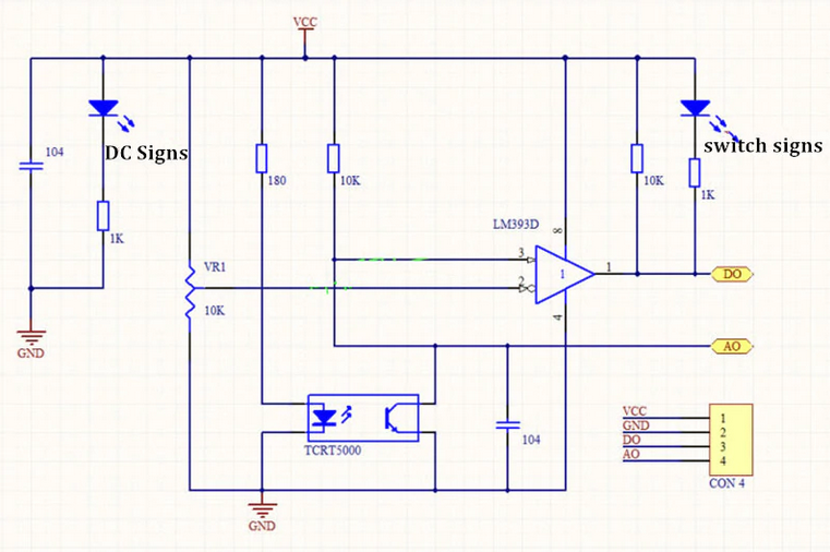
Image source: https://osoyoo.com/2017/08/15/tcrt5000-infrared-line-tracking-sensor/
To interpret the output value, study the following characteristic curve.
- Over a dark line: little IR returns, the phototransistor is off, and the analog output voltage is high.
- Over a white (reflective) surface: more IR returns, the phototransistor conducts, and the analog output voltage is low (near ground on A0).
Discuss the slope of the curve and the usable range for your application.
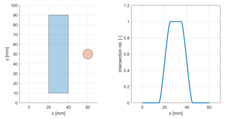
Differential sensor usage
Consider using two line sensors in a differential configuration. Treat one sensor as positive and the other as negative. With a clever placement, summing their outputs gives a good estimate of the robot’s lateral position relative to the line.

What about the gap between sensors? How does it affect the line‑following behavior?
Line node implementation
Implement a LineNode class that receives data and encapsulates the line estimation for the rest of the program.
- Create new files according to your project’s conventions.
- Subscribe to the topic
/bpc_prp_robot/line_sensors. - Message type:
std_msgs::msg::UInt16MultiArray.
// Public API sketch; adapt to your project
enum class DiscreteLinePose {
    LineOnLeft,
    LineOnRight,
    LineNone,
    LineBoth,
};

class LineNode : public rclcpp::Node {
public:
    LineNode();
    ~LineNode();

    // Relative pose to line [m]
    float get_continuous_line_pose() const;

    DiscreteLinePose get_discrete_line_pose() const;

private:
    rclcpp::Subscription<std_msgs::msg::UInt16MultiArray>::SharedPtr line_sensors_subscriber_;

    void on_line_sensors_msg(const std_msgs::msg::UInt16MultiArray::SharedPtr& msg);

    float estimate_continuous_line_pose(float left_value, float right_value);

    DiscreteLinePose estimate_discrete_line_pose(float l_norm, float r_norm);
};
Run the program and print the measured values for verification.
Line position estimation (1 h)
Now focus on estimating the line position. Create a class that encapsulates the algorithm. Inputs are left and right sensor values. Outputs are both the discrete and continuous position of the robot relative to the line.
Use test‑driven development (TDD): write tests first, then implement the algorithm.
// Minimal GTest example for a line estimator
#include <cstdint>
#include <gtest/gtest.h>

TEST(LineEstimator, BasicDiscreteEstimation) {
    uint16_t left_value = 0;
    uint16_t right_value = 1024;
    auto result = LineEstimator::estimate_discrete(left_value, right_value);
    EXPECT_EQ(result, /* expected pose */);
}

int main(int argc, char **argv) {
    ::testing::InitGoogleTest(&argc, argv);
    return RUN_ALL_TESTS();
}
By separating the algorithm into its own class, you make testing easier than embedding the logic directly inside LineNode.
Discrete approach
Provide a method that returns a discrete position relative to the line.
class LineEstimator {
public:
    static DiscreteLinePose estimate_discrete_line_pose(uint16_t left_val, uint16_t right_val);
};
Continuous approach
Do the same for the continuous case. Use raw sensor values as input and return a floating‑point lateral offset. Tip: scale the output to SI units [m].
class LineEstimator {
public:
    static float estimate_continuous_line_pose(uint16_t left_val, uint16_t right_val);
};
Line sensor calibration and arrangement (1 h)
Now review the physical sensor setup. On each robot, sensors may be mounted slightly differently (position, rotation, height above ground, wiring, resistor values, ICs, etc.).
At the start of a run, calibrate the sensors so the algorithm receives comparable values.
How to calibrate the sensor
Capture the minimum and maximum response (min reflection vs. max reflection) and normalize the output so your algorithm always works in the same range.
auto calibrated = (raw - min_val) / (max_val - min_val);
Clamp the normalized value to [0.0, 1.0].
Sensor arrangement
There are several mounting options on the robot. Consider how sensor position, field of view, and dynamic range influence your line‑following algorithm.
- What about the dead zone between sensors?
- What if sensors are too close to each other?
- Should one sensor be amplified relative to the other?
Lab 6 - Line Following & PID
Responsible: Ing. Petr Šopák
Learning objectives
- Bang-Bang Line Following (ON/OFF Control)
- Line Following with P-Control
- Line Following with PID Control
In previous lab sessions, you developed ROS 2 nodes for:
- Collecting data from reflection-based sensors
- Estimating the position of a line
- Controlling the robot's motion
Now, your task is to develop a strategy for line following – that is, responding to the estimated line position and ensuring the robot tracks the line correctly. You will start with the simplest approach (Bang-Bang control) and progressively refine it to implement PID regulation.
For more details, see the Line following chapter: Line following.
Bang-Bang Line Following (Approx. 1 hour)
Bang-Bang is the most basic control method. Instead of smoothly adjusting the speed, the robot makes hard, discrete decisions based on sensor readings. Think of it as a light switch – either ON or OFF:
- Line is detected on the left → Turn right
- Line is detected on the right → Turn left
- Line is centered → Move straight
This method can be implemented using either digital or analog sensor outputs. Since digital outputs already behave like ON/OFF signals, Bang-Bang logic is straightforward. However, in this lab, we will focus on the analog output, which requires setting a threshold to decide when the robot should turn.
The entire algorithm is illustrated in Figure 1. The process consists of reading the estimated line position and comparing it to a user-defined threshold. Based on this comparison, the robot's movement is determined.
The flowchart provides a generalized structure for Bang-Bang control. However, the specific comparison logic and the velocity values sent to the wheels depend on your own implementation. It is up to you to decide how to structure the control logic in your code.
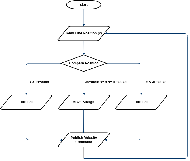
Figure 1: Flowchart for Bang-Bang Control
To fine-tune the performance, it is recommended to start with a higher threshold and gradually decrease it. Observe how the robot’s behavior changes and try to understand why this approach leads to better results.
TASK 1
- Project Structure:
- Inside the
srcandincludedirectories, create a new folder namedloops. - In this folder, create two files:
line_loop.cppandline_loop.hpp. - These files will define a ROS 2 node that implements a periodic control loop using a timer callback (e.g.,
line_loop_timer_callback()). - The loop should regularly read the estimated line position, compute the control action, and send appropriate speed commands to the robot's motors.
- Implement Bang-Bang Line Control based on the guidelines provided in the lab description.
- Experiment with different threshold values and observe how the robot behaves and analyze the advantages and limitations of Bang-Bang control.
Line Following with P-Control (Approx. 1 hour)
Now you will refine your line-following strategy by implementing Proportional Control (P-Control). Unlike Bang-Bang control, which causes abrupt movements, P-Control allows the robot to adjust its movement smoothly based on how far the estimated line position deviates from the robot’s center. The goal is to achieve smoother and more stable tracking of the line.
Previously you implemented Bang-Bang control, which relied on strict ON/OFF decisions. This approach worked but led to oscillations and jerky movement, as the robot continuously switched between turning left and right. These issues make it difficult for the robot to follow curves or move efficiently at higher speeds.
Proportional control solves this by introducing a continuous adjustment to the robot’s turning speed. Instead of making binary decisions, the angular velocity ω is determined using a proportional gain KP and the error e, which represents the difference between the estimated line position x and the robot's center x0:
$$ e = x - x_{0} $$
By multiplying this error by KP, we obtain the angular velocity:
$$ ω = K_{P} \cdot e $$
This means that when the robot is far from the center, it turns more sharply. When it is close to the center, it makes minor corrections. If the line is perfectly centered, the robot moves straight. The higher the proportional gain KP, the stronger the response to the error. However, if KP is too high, the robot may start oscillating.
The process of P-Control is illustrated in Figure 2. The robot reads the estimated position of the line, calculates the error, applies the proportional formula to determine angular velocity, and then sends this velocity to the motion control node, which executes the movement.
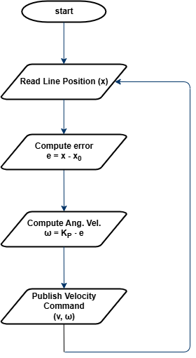
Figure 2: Flowchart for P-Control Line Follower
A key part of implementing P-Control is choosing the right value for KP. If KP is too small, the robot will react very slowly and may fail to follow the line accurately. If KP is too large, the robot might oscillate too much and become unstable. The best approach is to start with a low value of KP and gradually increase it, observing how the robot’s movement improves.
TASK 2
- Insert the provided
pid.hppfile into theinclude/algorithmsdirectory. This header defines a basic PID controller class, which you will use for both Task 2 (P-control) and Task 3 (full PID).
#pragma once

#include <iostream>
#include <chrono>

namespace algorithms {

    class Pid {
    public:
        Pid(float kp, float ki, float kd)
            : kp_(kp), ki_(ki), kd_(kd), prev_error_(0), integral_(0) {}

        float step(float error, float dt) {
            integral_ += error * dt;
            float derivative = (error - prev_error_) / dt;
            float output = kp_ * error + ki_ * integral_ + kd_ * derivative;
            prev_error_ = error;
            return output;
        }

        void reset() {
            prev_error_ = 0;
            integral_ = 0;
        }

    private:
        float kp_;
        float ki_;
        float kd_;
        float prev_error_;
        float integral_;
    };
}
- Reuse your
LineLoopclass from Task 1 and modify the control logic insideline_loop_timer_callback()to implement a Proportional controller. - Experiment with different values of the proportional gain KP and determine the most suitable value.
- Observe the performance and assess if further refinement is needed.
- Write simple unit tests for the
Pidclass in a separate file namedpid_test.cpp. Here's an example that tests the response of the P-controller to a unit step input:
#include "algorithms/pid.hpp"
#include <iostream>
#include <cassert>
#include <cmath>

using namespace algorithms;

bool nearly_equal(float a, float b, float eps = 1e-5f) {
    return std::fabs(a - b) < eps;
}

// Unit step input (constant error = 1.0)
void test_unit_step() {
    Pid pid(2.0f, 0.0f, 0.0f); // P-only
    float dt = 0.1f;

    float error = 1.0f;

    for (int i = 0; i < 5; ++i) {
        float output = pid.step(error, dt);
        assert(nearly_equal(output, 2.0f));
    }

    std::cout << "[PASS]\n";
}

int main() {
    test_unit_step();

    std::cout << "All P-controller tests passed.\n";
    return 0;
}
Line Following with PID Control (Approx. 1 hour)
In this part, you will refine your P-Control implementation by adding Integral (I) and Derivative (D) components, creating a PID controller. This will improve stability, reduce oscillations, and enhance the robot’s ability to follow curves accurately.
While P-Control adjusts the robot’s angular velocity based on the current error, it does not account for past errors or predict future corrections. This can result in oscillations or slow responses in certain situations. PID control solves these issues by incorporating two additional terms:
$$ ω = K_{P}e + K_{i}\int e dt + K_{d}\frac{de}{dt} $$
- $$K_{P}e$$ (Proportional term): Reacts to the current error.
- $$K_{i}\int e dt$$ (Integral term): Corrects accumulated past errors.
- $$K_{d}\frac{de}{dt}$$ (Derivative term): Predicts future errors and reduces overshooting.
The integral term helps eliminate steady-state errors, ensuring the robot remains centered over time. The derivative term improves responsiveness by counteracting rapid changes, preventing overshooting and oscillations.
The overall process is illustrated in Figure 3. The robot reads the estimated line position, computes the error, applies the PID formula, and sends the adjusted velocity command to the motion control node.
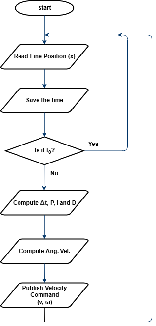
Figure 3: Flowchart for PID Control
Tuning KP, Ki, Kd is essential for optimal performance. If KP is too high, the robot may oscillate. If Ki is too high, the robot may overcorrect. If Kd is too high, the robot may become too sensitive to small errors. A common approach is to start with only KP, then add Kd, and finally add Ki to eliminate steady-state error.
For more information on PID control implementation and tuning methods, see PID.
TASK 3
- Just like in the previous tasks, extend your
LineLoopclass to implement full PID control using the providedPidclass. Also, don’t forget to extend your unit tests (pid_test.cpp) to verify the behavior of all PID components. - Choose a tuning method (either manual tuning or the Ziegler-Nichols method) and find the optimal values for KP, Ki, Kd.
- Observe the differences between PID control and the previous line-following methods. Analyze how each component affects the robot’s performance.
- (Optional) Implement output saturation (clamping). Real robots cannot turn infinitely fast. If your PID controller outputs a very large value (e.g. due to a sharp error), you should limit (saturate) it to a safe range.
- (Optional) Implement anti-windup. The integral term in a PID controller can sometimes accumulate too much (especially when the output is saturated), which leads to overshooting or instability. This is called integral windup. To prevent this, implement anti-windup, for example disabling integration when output is saturated or limiting the maximum integral value.
Lab 7 - Midterm Test (Line Following)
Responsible: Ing. Adam Ligocki, Ph.D.
Up to 50 points can be earned through two practical demonstrations during the semester.
Week 7 — Line following (20 points)
Week 12 — Corridor following (20 points)
Line following rules
There are 3 tracks:
- Straight line (5 points)
- Simple loop (5 points)
- Complex loop (10 points)
To pass a track, the robot must follow the full length of the line.
If no part of the robot's body covers the line, the attempt fails.
Points are awarded only for completing the entire track.
Teams have 3 attempts per track, with a time limit of 3 minutes per attempt.
All 3 attempts must be performed during a single lab session.
Test tracks

Lab 8 - Obstacle Detection & Corridor Following
Responsible: Ing. Petr Šopák
Learning objectives
1) Understanding and working with LiDAR and/or Ultrasonic Sensors
- Interpreting range data based on sensor principles
- Visualizing live sensor output in RViz2
2) Implementing basic Obstacle Detection
- Detecting nearby obstacles
- Implementing basic obstacle avoidance strategy
3) Implementing corridor following behavior
In the previous labs, you implemented line following — the robot follows a visible line on the floor. This method is useful in controlled environments, such as factory floors or predefined paths. However, line following relies on the presence of artificial markings and provides limited flexibility in more general environments.
In this and the next labs, you will begin working on corridor following, a more natural and scalable navigation strategy. Instead of relying on a line, the robot uses range sensors (LiDAR or ultrasonic) to perceive the environment and stay centered between two walls or obstacles, like navigating a hallway. This approach is closer to what real autonomous robots do in indoor spaces, such as offices, hospitals, or warehouses.
You will first learn how to interpret range data and detect nearby obstacles. Then, you will implement a simple reactive controller that enables the robot to stay within a corridor.
Understanding and working with LiDAR and/or ultrasonic sensors (Approx. 40 minutes)
In this part of the lab, you will get familiar with your chosen range sensor — either LiDAR or ultrasonic. You will explore how it measures distance, how the data is represented in ROS 2, and how to visualize it in RViz2. This will give you the foundation needed for obstacle detection and corridor following tasks in the rest of the lab.
For these labs, please choose one type of range sensor — either ultrasonic or LiDAR. You will work with the selected sensor throughout the exercises. If you later decide to switch to the other sensor or want to use both for comparison or improvement, feel free to do so. The instructions are written to support both sensor types.
A) Light Detection and Ranging (LiDAR) sensor
LiDAR sensors are commonly used in robotics to measure precise distances to surrounding objects. A LiDAR device emits rapid laser pulses and measures the time it takes for each pulse to bounce back from a surface. Using the known speed of light, it calculates the exact distance to each point. Most LiDARs used in mobile robots operate in 2D, scanning a horizontal plane around the robot to produce a range profile of the environment. This allows the robot to detect walls, obstacles, and open spaces with high accuracy and resolution.
When implementing the tasks, please refer to the official documentation of the sensor. You can find the RPLIDAR A1 datasheet here: RPLIDAR A1 datasheet
TASK 1 - A
- Explore the data provided by the sensor - Inspect the raw data in the terminal (Refer to the datasheet if needed to understand parameters)
Understand the meaning of the main fields in the message:
angle_min,angle_max,angle_increment,ranges[],range_max,range_min. - Visualize the LiDAR data in RViz2
- Launch RViz2 and add a LaserScan display (Add → By Topic → LaserScan)
- Set the correct topic name and
Fixed Frameaslidar - (Optional) Customize the display: point size, color, decay time, etc.
Don’t forget to launch RViz2 in a sourced terminal; otherwise topics will not be visible.
- Create a new
ROS 2node for your LiDAR processing- Create
lidar_node.hppandlidar_node.cppinnodesdirectories - In this node, subscribe to the LiDAR topic and process incoming data
- Create
- Think critically about the data
- Are all values in
ranges[]useful for your application?
TIP: LiDAR may return very small values (e.g. 0) or extremely large values (inf). These are usually best ignored.
- Do all directions matter for your robot’s task?
TIP: You can filter only specific angular sectors depending on what you need. (e.g. Front, Right, Left, Back)
- (Optional) Example skeleton for implementing sector-based LiDAR filtering. You may use this as inspiration or create your own version:
#include <cmath> #include <vector> #include <numeric> namespace algorithms { // Structure to store filtered average distances in key directions struct LidarFilterResults { float front; float back; float left; float right; }; class LidarFilter { public: LidarFilter() = default; LidarFilterResults apply_filter(std::vector<float> points, float angle_start, float angle_end) { // Create containers for values in different directions std::vector<float> left{}; std::vector<float> right{}; std::vector<float> front{}; std::vector<float> back{}; // TODO: Define how wide each directional sector should be (in radians) constexpr float angle_range = ; // Compute the angular step between each range reading auto angle_step = (angle_end - angle_start) / points.size(); for (size_t i = 0; i < points.size(); ++i) { auto angle = angle_start + i * angle_step; // TODO: Skip invalid (infinite) readings // TODO: Sort the value into the correct directional bin based on angle } // TODO: Return the average of each sector (basic mean filter) return LidarFilterResults{ .front = , .back = , .left = , .right = , }; } }; } - Are all values in
B) Ultrasonic sensors
Ultrasonic sensors are widely used in robotics for short-range obstacle detection. They work by emitting a high-frequency sound wave and measuring the time it takes for the echo to return after bouncing off an object. Unlike LiDAR, ultrasonic sensors typically measure in a narrow cone, and their readings can be affected by surface material, angle, or ambient noise. They are cost-effective, but require more filtering and careful placement to be reliable.
When implementing the tasks, please refer to the official documentation of the sensor. You can find the HY-SRF05 datasheet here: HY‑SRF05 datasheet
TASK 1 - B
- Explore the data provided by the sensor — Inspect the raw data in the terminal (refer to the datasheet if needed to understand parameters — min/max measurable range, FOV, etc.)
- Visualize the data in rqt (or RViz2 — use the Range display)
- Create a new ROS 2 node for processing ultrasonic data
- Create
ultrasonic_node.hppandultrasonic_node.cppinnodesdirectories - In this node, subscribe to the topic and process incoming data
- Create
- Think critically about the data
- What do the sensor values actually represent?
- Are the sensor readings stable and consistent over time?
TIP: Data is often affected by noise, reflections, and material properties. You may want to ignore extreme or invalid values. Consider applying filtering, such as a moving average or median filter
- If needed, implement a simple filtering algorithm to reduce noise or focus only on relevant angles (e.g. front, sides)
Implementing basic Obstacle Detection (Approx. 40 minutes)
Use your chosen sensor (LiDAR or ultrasonic) to detect whether an object is too close to the robot — for example, less than 0.30 m in front. If an obstacle is detected, the robot should stop and wait instead of continuing forward. This simple reactive behavior is an essential first step toward more advanced navigation strategies such as obstacle avoidance, corridor following, or autonomous path planning.
TASK 2
- Create a new ROS 2 node called
corridor_loopin theloopsdirectory. This node should be similar to theline_loopfrom the previous labs. In this node, you will gradually implement the entire functionality for Corridor Following - Use the sensor data from Task 1. Based on this data, implement a simple algorithm for Obstacle Detection:
- Retrieve the data from the sensors
- If the reading is below a threshold you define, this means the robot is close enough to detect the obstacle
- Test the obstacle detection to ensure the robot detects objects correctly when they are within the defined range.
- Create basic obstacle avoidance logic:
- Make the robot drive forward
- When an obstacle is detected, the robot must stop and not continue moving!
More advanced avoidance behaviors (e.g., turning) will be covered in the next lab.
Implementing corridor following behavior (Approx. 60 minutes)
Corridor following allows the robot to stay centered between two walls by adjusting its heading based on distance measurements from both sides. In this task, you will use your sensor data (e.g. LiDAR or ultrasonic) to calculate the lateral error (difference between left and right distances) and correct the robot’s trajectory using proportional control.
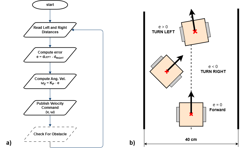
Figure 1: Corridor following behavior. a) Flowchart of the corridor following algorithm; b) Robot behavior based on the computed lateral error e.
TASK 3
- Implement the corridor-following algorithm based on the flowchart displayed above.
- Test and tune the algorithm to find the optimal solution for corridor following. (You may use the
pid.hppfor advanced control if desired.)
Note: It is recommended to test corridor following in environments where the turns are not too sharp. This issue will be addressed in the next lab.
Lab 9 – Orientation-Aware Corridor Navigation
Responsible: Ing. Petr Šopák
Learning objectives
1) Understanding robot orientation using IMU (MPU6050)
- Interpreting raw gyroscope data
- Calibrating and integrating gyro values to estimate yaw
2) Extending corridor following with corner handling
- Detecting turns (e.g. 90° corners) using range sensors
- Executing rotation using IMU feedback
3) Implementing a state-based navigation strategy
- Designing a simple state machine
- Switching between corridor following and turning behavior
Introduction
In Lab 9, you implemented a basic reactive controller that allowed the robot to follow straight corridors using range sensors such as LiDAR or ultrasonic. However, this approach assumes that the path is straight and cannot handle corners or sharp turns.
In this lab, you will enhance that behavior by enabling your robot to detect and turn into new corridor directions (e.g., 90° left or right turns). To accomplish this, you will use an Inertial Measurement Unit (IMU) — specifically the MPU‑6050 (MPU‑6050 datasheet) — to estimate the robot's yaw (rotation around the vertical axis).
The robot will:
- Follow the corridor as before
- Detect the corner
- Rotate in place until it is aligned with the new corridor direction
- Resume forward motion
To implement this, you will also develop a simple finite state machine with at least two states: CORRIDOR_FOLLOWING and TURNING.
IMU and orientation estimation (Approx. 70 minutes)
The MPU6050 sensor provides raw data from a gyroscope and accelerometer. Unlike more advanced IMUs, it does not provide direct orientation estimates such as yaw, pitch, or roll.
To estimate yaw (rotation angle), you will:
- Read the raw gyroscope value for the z-axis (
gyro_z), which represents angular velocity around the vertical axis. - Calibrate:
- Keep the robot still for 2–5 seconds after startup.
- Collect multiple
gyro_zvalues. - Compute the average value as the
gyro_offset.
- Integrate over time:
- Subtract the offset from each reading.
- Multiply by the time delta (
dt) to obtain the yaw angle increment. - Accumulate this over time to estimate the current yaw:
yaw += (gyro_z - offset) * dt;
Practical Integration Tip
In this lab, you are required to implement the yaw integration yourself. No sensor fusion libraries will be used. Keep in mind that this method is sensitive to drift, so proper calibration is critical.
Corner Detection
When following a corridor, the robot can monitor the side range sensors. If a wall suddenly "disappears" on one side (i.e., the distance becomes much larger), and the front is also open, it likely means the corridor turns in that direction.
An alternative strategy is to detect a wall in front of the robot (i.e., front distance drops below a defined threshold), and then search for an opening on the sides to determine where the corridor continues. However, this method is problematic in case of intersections, as the robot may overshoot the corner and fail to turn properly.
TASK 1 – IMU Integration and Yaw Estimation
- Create a new ROS 2 node for the IMU (e.g., imu_node)
- Subscribe to the MPU6050 data and read
gyro_zvalues from the topic. A suggested node structure and a helper class are provided below this task - Implement gyroscope calibration:
- At the beginning of the program, keep the robot completely still for 2–5 seconds
- During this time, collect several
gyro_zvalues. - Compute the average of these samples to obtain the gyroscope offset
gyro_offset.
You will subtract this offset from all future gyro readings to reduce drift
- Estimate yaw (heading):
- In a timed loop, Subtract the
gyro_offsetfrom the currentgyro_zvalue to get the corrected angular velocity - Multiply the corrected value by the time delta
dtto get the yaw increment - Accumulate this increment into a variable yaw that represents the current robot orientation (the formula was described before)
- In a timed loop, Subtract the
- Test IMU-based yaw estimation and implement basic heading correction
- Manual Rotation test
- Calibrate the IMU and store the current yaw
- Pick up or gently rotate the robot by approximately 90° (by hand)
- The robot should detect the yaw error:
float yaw_error = yaw_ref - current_yaw; - If the error exceeds a threshold (e.g. 5°), apply a corrective rotation using differential motor speeds:
float correction = Kp * yaw_error; motor_node->set_motor_speed(127 - correction, 127 + correction); - The robot should rotate back toward its original orientation
- External Disturbance test
- While the robot is driving straight or standing still, apply a light push to rotate it
- The robot should detect the change in yaw and try to rotate back to its original heading based on the integrated yaw
Always calibrate the IMU at the beginning — without proper calibration, even small disturbances will cause significant drift over time!
- Manual Rotation test
Example of imu_node.hpp:
#include <rclcpp/rclcpp.hpp>
#include <sensor_msgs/msg/imu.hpp>
#include "algorithms/planar_imu_integrator.hpp"

namespace nodes {

    enum class ImuNodeMode {
        CALIBRATE,
        INTEGRATE,
    };

    class ImuNode : public rclcpp::Node {
    public:
        ImuNode();
        ~ImuNode() override = default;

        // Set the IMU mode
        void setMode(ImuNodeMode mode);

        // Get the current IMU mode
        ImuNodeMode getMode();

        // Get the results after integration
        auto getIntegratedResults();

        // Reset the class
        void reset_imu();

    private:

        void calibrate();
        void integrate();

        ImuNodeMode mode = ImuNodeMode::INTEGRATE;

        rclcpp::Subscription<sensor_msgs::msg::Imu>::SharedPtr imu_subscriber_;
        algorithms::PlanarImuIntegrator planar_integrator_;

        std::vector<float> gyro_calibration_samples_;

        void on_imu_msg(const sensor_msgs::msg::Imu::SharedPtr msg);
    };
}
To simplify your IMU logic, use a helper class planar_imu_integrator.hpp to encapsulate yaw estimation. If you later want to include velocity or position tracking, you’ll need to extend the structure. (Don't forget to write the tests)
#include <iostream>
#include <cmath>
#include <numeric>

namespace algorithms {

    class PlanarImuIntegrator {
    public:

        PlanarImuIntegrator() : theta_(0.0f), gyro_offset_(0.0f) {}

        // TODO: Call this regularly to integrate gyro_z over time
        void update(float gyro_z, double dt);

        // TODO: Calibrate the gyroscope by computing average from static samples
        void setCalibration(std::vector<float> gyro);

        // TODO: Return the current estimated yaw
        [[nodiscard]] float getYaw() const;

        // TODO: Reset orientation and calibration
        void reset();

    private:
        float theta_;       // Integrated yaw angle (radians)
        float gyro_offset_; // Estimated gyro bias
    };
}
State machine for corridor navigation (Approx. 70 minutes)
If you have implemented the IMU, you are now ready to extend your corridor-following behavior. In this lab, you will implement a simple state machine to structure the robot's behavior during navigation. Instead of relying on a single control strategy, your robot will dynamically switch between multiple modes:
- CALIBRATION – the robot stays still and computes IMU offset before navigation begins
- CORRIDOR_FOLLOWING – the robot drives straight and uses side range sensors to stay centered between walls
- TURNING – the robot rotates in place using the IMU until a 90° turn is completed
- (Later additions:) INTERSECTION_HANDLING, DEAD_END_HANDLING, etc.
This modular architecture will make your logic easier to extend in future — for example, adding states INTERSECTION_HANDLING (two or three paths), DEAD_END_HANDLING (dead end).
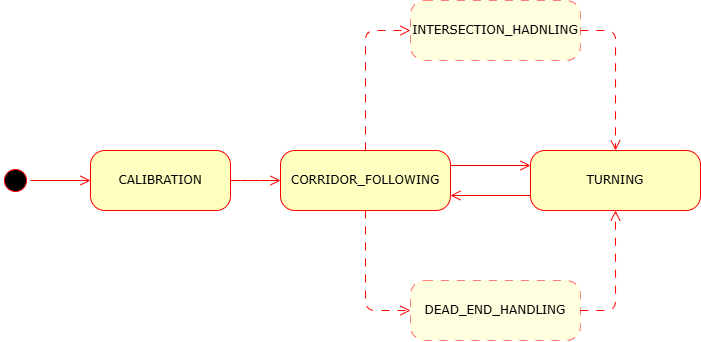
Figure 1: Example state diagram for corridor-following behavior
Notes:
- The structure below is just an example. You are free to design your own solution — don’t feel limited by this template!
- Keep your implementation modular so it can be extended in future
- Always calibrate the IMU at startup to avoid drift in yaw estimation
TASK 2 - Implementing Corner Detection and Turning
- In your corridor loop node, integrate the state machine logic
- Example Structure:
 switch (state) {
  case CALIBRATION:
 // Wait until enough samples are collected
 // Once done, switch to CORRIDOR_FOLLOWING
 break;

   case CORRIDOR_FOLLOWING:
     // Keep centered using P/PID based on side distances
     // If front is blocked and one side is open → switch to TURNING
     break;

   case TURNING:
     // Use IMU to track rotation
     // Rotate until yaw changes by ±90°
     // Then return to CORRIDOR_FOLLOWING
     break;
 }
- Example Structure:
- In the
CORRIDOR_FOLLOWINGstate:- Use side range sensor data to stay centered between walls.
- Monitor the front sensor: if the front distance falls below a threshold (e.g., < 0.10 m) and one side is open, detect a corner
- Based on which side is open, decide the direction to turn (left or right)
- Switch to the
TURNINGstate
- In the
TURNINGstate:- Store the current yaw as
yaw_start - Command the robot to rotate
- Continuously read yaw and compare with
yaw_start - When the yaw change reaches ~90°, stop the rotation and switch back to
CORRIDOR_FOLLOWING
- Store the current yaw as
Lab 10 - Visual Navigation Using ArUco Markers
Responsible: Ing. Petr Šopák
Learning objectives
1) Camera-based detection of visual markers
- Subscribing to a camera image topic
- Converting ROS image messages to OpenCV format
- Detecting ArUco markers using a provided detector
2) Using markers for high-level decision making
- Associating marker IDs with semantic instructions (e.g., “turn left”, “goal”)
- Storing and reusing symbolic information
- Implementing logic that uses past observations during navigation
Requirements
For this lab, you need to have the image transport plugins package installed:
sudo apt update
sudo apt install ros-humble-image-transport-plugins -y
To check all available transport plugins, run:
ros2 run image_transport list
You should see an output similar to:
Declared transports:
image_transport/compressed
image_transport/compressedDepth
image_transport/raw
image_transport/theora

Details:
...
Introduction
In previous labs, you explored sensor-based navigation using range sensors and IMUs. These approaches allowed the robot to react to its surroundings, but they did not provide access to symbolic information or long-term guidance.
In this lab, your robot will navigate through a maze where ArUco markers act as visual hints. These markers are placed at strategic locations and convey semantic instructions, such as which direction to take at an intersection, or where a shortcut to a goal (e.g., treasure) can be found.
The robot’s goal is to detect the markers, interpret their meaning, and use this information later when making decisions in the maze. This symbolic memory allows the robot to act in a more informed and efficient way, rather than relying solely on reactive behaviors.
Camera and Marker Detection (Approx. 50 minutes)
In the first part of the lab, you will implement a ROS 2 node (CameraNode) that subscribes to a camera image stream, converts the received image into OpenCV format, and detects ArUco markers.
You are provided with a partial implementation of the ArucoDetector class. Your task is to complete this class and integrate it into your ROS node.
TASK 1 – Camera Subscription and Marker Detection
- Create a new ROS 2 node -
camera_node- Subscribe to a camera image topic (
/bpc_prp_robot/camera/compressed) usingsensor_msgs/msg/compressed_image.hpp - In the callback, decode the incoming compressed image message using
cv::imdecodeto obtain acv::MatinBGRformat (equivalent tobgr8) - Check if the decoded image is valid (not empty) before processing
- Subscribe to a camera image topic (
- Detect ArUco markers in the image:
- Use the provided
aruco_detector.hpp(insert it toalgorithmsfolder) and complete the class - The detector will return a list of marker IDs and corner coordinates
 #include <opencv2/opencv.hpp>
 #include <opencv2/aruco.hpp>

 namespace algorithms {

     class ArucoDetector {
     public:

         // Represents one detected marker
         struct Aruco {
             int id;
             std::vector<cv::Point2f> corners;
         };

         ArucoDetector() {
             // Initialize dictionary with 4x4 markers (50 possible IDs)
             dictionary_ = cv::aruco::getPredefinedDictionary(cv::aruco::DICT_4X4_50);
         }

         ~ArucoDetector() = default;

         // Detect markers in the input image
         std::vector<Aruco> detect(cv::Mat frame) {
             std::vector<Aruco> arucos;

             std::vector<int> marker_ids;
             std::vector<std::vector<cv::Point2f>> marker_corners;

             // TODO: Detect markers using OpenCV
             // cv::aruco::detectMarkers(...);

             if (!marker_ids.empty()) {
                 std::cout << "Arucos found: ";
                 for (size_t i = 0; i < marker_ids.size(); i++) {
                     std::cout << marker_ids[i] << " ";

                     // TODO: Create Aruco struct and add to result vector
                     // arucos.emplace_back(...);
                 }
                 std::cout << std::endl;
             }

             return arucos;
         }

     private:
         cv::Ptr<cv::aruco::Dictionary> dictionary_;
     };
 }
- Use the provided
- Store the last frame and detection results:
- Save the latest image (
cv::Mat) and detection data (std::vector<Aruco>)
- Save the latest image (
- Visualize the incoming camera stream
- Publish the (optionally annotated) image using
image_transport::Publisher - View the image in rqt_image_view or RViz for debugging
RViz2 tip: Add → By Topic → Image, then set Image Topic (in Displays) to
/bpc_prp_robot/camera/compressed- (Optional) Overlay detected markers on the image using
cv::aruco::drawDetectedMarkersbefore publishing
- Publish the (optionally annotated) image using
Symbolic Navigation Logic (Approx. 40 minutes)
In the second part of the lab, you will design logic that interprets the detected ArUco markers as instructions for maze navigation. Some markers indicate directions that lead to the exit, while others point toward the treasure. Your robot must recognize and remember these instructions, and then apply them later at decision points.
As illustrated in Figure 1, each instruction obtained from an ArUco marker is always intended for the next upcoming intersection. The robot must remember the marker’s content and apply it at the first junction it encounters after reading the marker.
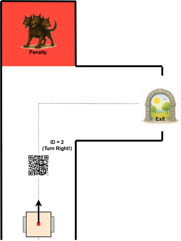
Figure 1: Example of decision-making using ArUco markers in a maze.
TASK 2 - Maze Logic and Decision Making
- In your maze loop node (or a separate logic node):
- Use the data obtained from the previous task
- Define a mapping between marker IDs and symbolic instructions (see table below)
- Remember that there are two types of markers: one for the exit path, and one for the treasure path
Escape path: Treasure Path: ID = 0 -> straight ID = 10 -> straight ID = 1 -> left ID = 11 -> left ID = 2 -> right ID = 12 -> right - Integrate the symbolic information into navigation logic
- When a marker is detected, store the ID and its meaning
- When the robot reaches the first intersection or decision point, use the stored instruction to select the direction
- Based on the instruction (e.g., turn left), command the robot to rotate and follow the chosen path
TIP: Define which path (escape or treasure) has higher priority
- Test your logic and outputs
Final note
This is the last lab in the course. We hope it helped you better understand the connection between perception, memory, and decision-making in robotics. You’ve now completed a full pipeline—from reading sensor data to interpreting symbolic cues and applying them in complex navigation tasks.
Good luck with your upcoming exam and final evaluation. Stay curious, keep experimenting, and don’t be afraid to challenge your solutions. We’ll be happy to see if you decide to join another course from our Robotics group in the future.
Lab 12 - Midterm Test (Corridor Following)
Responsible: Ing. Adam Ligocki, Ph.D.
Up to 50 points can be earned through two practical demonstrations during the semester.
Week 7 — Line following (20 points)
Week 12 — Corridor following (20 points)
Corridor following rules
There are 3 tracks:
- Straight corridor (5 points)
- Simple loop (10 points)
- Complex loop (10 points)
The corridor is defined by walls.
All tracks use a rectangular grid of 0.40 × 0.40 m.
Cells are marked by black tape on the ground.
Points are awarded only for completing the entire track:
- Pass the straight corridor without touching the wall.
- Complete the full loop.
- Do not touch the walls.
- Do not enter the same cell more than once.
Teams have 3 attempts per track, with a time limit of 3 minutes per attempt.
All 3 attempts must be performed during a single lab session.
Test tracks
- Walls: red lines
- Path: green line
- Start: green cell
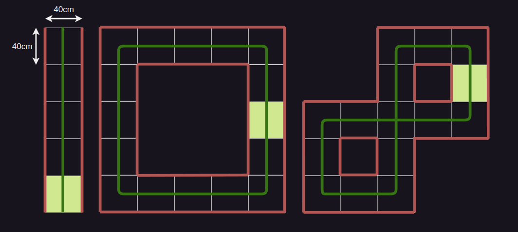
Final Exam - Maze Escape
Responsible: Ing. Adam Ligocki, Ph.D.
The final exam is a competition. Each team has up to 3 attempts to escape the maze using the robot’s sensors. The final score is based on the best attempt.
- The robot starts in the center of the starting cell.
- There is one optimal escape path.
- The maze contains no loops.
- There are 3 randomly placed minotaurs and 1 treasure.
- Each minotaur encounter adds a 30 s penalty.
- Finding the treasure subtracts 30 s from the final time.
- The maze consists of 8 × 8 cells; each cell is 0.40 × 0.40 m. Black tape on the floor marks the boundaries between cells.
- ArUco tags are placed on the floor and provide hints about the escape route, minotaurs, or treasure.
Scoring
In total, a team can earn up to 50 points:
- Maze escape: up to 40 points.
- Score is calculated as
y = min(max(kx + q, 0), 40).
- Score is calculated as
- Git and project documentation quality: up to 10 points.
Attempt rules
- Teams have at least 45 minutes between attempts to modify their program.
- The competition code must be uploaded to Git by 23:59 on the same day.
- The competition code must not contain specific information about the maze (e.g., paths, minotaur locations). Pre‑known constants (e.g., cell size) may be included.
- Do not touch the walls.
Maze example
- Walls: red lines
- Escape path: green line
- Start: green cell
- Treasure (bonus): blue cell
- Minotaur (penalty): red cell
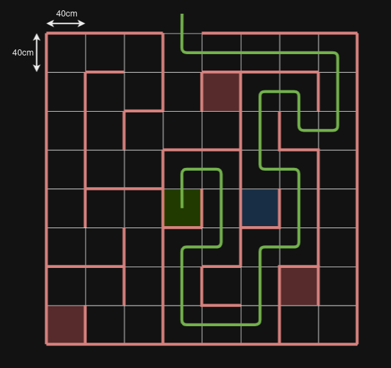
Navigation
Differential Chassis
The differential drive chassis is one of the most common configurations for mobile robots. It consists of two independently controlled wheels mounted on the same axis and optionally a passive caster wheel for stability.
This tutorial introduces the fundamental concepts of differential drive kinematics and demonstrates how to derive the forward and inverse kinematics equations.
Components of a Differential Drive Chassis
- Two wheels: Independently driven, providing linear and rotational motion.
- Chassis: Holds the wheels, motors, and sensors.
- Center of the robot: Defined as the midpoint between the two wheels.
- Wheel radius (
r): Radius of each wheel. - Wheel separation (
L): Distance between the two wheels.
Kinematic Model
Pose (x,y,θ): The robot's position (x,y) and orientation θ in a 2D plane. [m, m, rad]
Linear velocity (v): Forward speed of the robot. [m/s]
Angular velocity (ω): Rate of rotation of the robot. [rad/s]
Conventions:
- Coordinate frame: x points forward, y points to the left (right-handed frame).
- Positive angular velocity
ωis counter-clockwise (CCW). - Wheel linear speeds
v_L,v_Rare positive when rolling forward.
Wheel Velocities
Left wheel angular velocity: ω_L
Right wheel angular velocity: ω_R
The linear velocities of the wheels are (v_L = r·ω_L, v_R = r·ω_R):
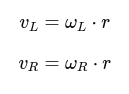
Forward Kinematics
Forward kinematics calculates the robot's linear and angular velocities based on wheel velocities.
Linear and Angular Velocities
The robot's linear velocity (v) and angular velocity (ω) are:
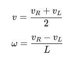
Turning radius and ICC
- Instantaneous Center of Curvature (ICC) lies at distance
R = v/ωfrom the robot center, to the left forω > 0and to the right forω < 0. - Special cases:
- Straight motion:
ω = 0→R = ∞. - In-place rotation:
v = 0,ω ≠ 0→R = 0(wheels spin in opposite directions with equal speed).
- Straight motion:
Pose Update
Given the robot's current pose (x,y,θ), the new pose after a small time step dt can be computed as:
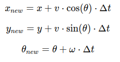
Inverse Kinematics
Inverse kinematics computes the wheel velocities required to achieve a desired linear and angular velocity.
Given:
- Desired linear velocity
v. - Desired angular velocity
ω.
The wheel velocities are:
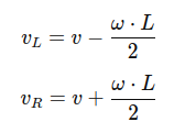
To compute angular velocities:
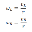
Example Code
def forward_kinematics(v_L, v_R, L):
    v = (v_R + v_L) / 2
    omega = (v_R - v_L) / L
    return v, omega
import math

def update_pose(x, y, theta, v, omega, dt):
    x_new = x + v * math.cos(theta) * dt
    y_new = y + v * math.sin(theta) * dt
    theta_new = theta + omega * dt
    # Optional: normalize heading to [-pi, pi)
    if theta_new > math.pi:
        theta_new -= 2 * math.pi
    elif theta_new <= -math.pi:
        theta_new += 2 * math.pi
    return x_new, y_new, theta_new
def inverse_kinematics(v, omega, L):
    v_L = v - (omega * L / 2)
    v_R = v + (omega * L / 2)
    return v_L, v_R
Exercise
Write a program that simulates a differential-drive chassis based on the given input parameters.
Simulation Parameters
- Wheel radius:
r = 0.1 m - Wheel separation:
L = 0.15 m - Time step:
dt = 0.01 s
Tasks
- Compute the pose of the robot after moving straight for 5 seconds with
v = 1 m/s. - Simulate a circular motion with
v = 1 m/sandω = 0.5 rad/s. - Simulate a circular motion with
v_L = 1.0 m/sandv_R = 0.5 m/s. - Optional: If using wheel angular speeds instead, compute
v_L = r·ω_Landv_R = r·ω_Rfirst.
PID
This tutorial introduces the concept of PID control and demonstrates how to implement it in a step-by-step manner, suitable for university-level students.
Proportional-Integral-Derivative (PID) control is one of the most widely used control algorithms in engineering and robotics. It is a feedback control mechanism used to maintain a desired setpoint by minimizing error in dynamic systems. PID controllers are found in applications ranging from industrial machinery to autonomous robots.
PID Basics
A PID controller continuously calculates an error value e(t), which is the difference between a desired setpoint r(t) and a measured process variable y(t):
The controller output u(t) is computed as:
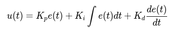
where:
Kpis Proportional gain.Kiis Integral gain.Kdis Derivative gain.
Proportional Control Kp:
Responds to the current error.
Larger Kp leads to a faster response but may overshoot.
Integral Control Ki
Responds to the accumulation of past errors. Helps eliminate steady-state error.

Derivative Control Kd
Responds to the rate of change of the error. Predicts future behavior and reduces overshoot.
PID Implementation
In digital systems, the continuous equation is approximated using discrete time intervals (dt):
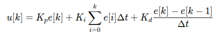
Algorithm
- Measure the current system output
y[k]. - Calculate the error:
e[k] = r[k] − y[k]. - Compute the proportional, integral, and derivative terms.
- Combine the terms to compute
u[k]. - Apply
u[k]to the system. - Repeat.
Example Code
class PIDController:

    def __init__(self, kp, ki, kd, setpoint=0.0, output_limits=(None, None), integral_limits=(None, None)):
        self.kp = kp
        self.ki = ki
        self.kd = kd
        self.setpoint = setpoint

        self.previous_error = 0
        self.integral = 0

    def update(self, measured_value, dt):
        error = self.setpoint - measured_value

        # P
        proportional = self.kp * error

        # I
        self.integral += error * dt
        integral = self.ki * self.integral

        # D
        derivative = self.kd * (error - self.previous_error) / dt

        self.previous_error = error
        output = proportional + integral + derivative
        return output
Practical Tips
- Keep units consistent and sample time Δt stable; prefer a monotonic time base.
- Start with small gains to avoid saturation; increase gradually.
- Set
output_limitsto your actuator range (e.g., PWM 0–255) and useintegral_limitsto prevent windup. - Consider computing the derivative on the measurement or apply a small low-pass filter to the D term if the signal is noisy.
- If the process variable is bounded (e.g., angle), consider wrapping errors appropriately.
PID Tuning
Manual Tuning
Start with Ki = 0 and Kd = 0.
Increase Kp until the system oscillates.
Increase Kd to dampen oscillations.
Introduce Ki to eliminate steady-state error.
Ziegler-Nichols Method
Set Ki=0 and Kd = 0.
Increase Kp until the system oscillates with constant amplitude.
Note the critical gain Ku and period Tu.
Set parameters as:
Kp = 0.6 * KuKi = 2 * Kp / TuKd = Kp * Tu / 8
Common Problems
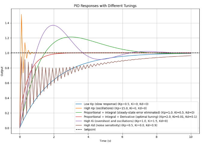
- Low
Kp(slow response): The system reacts very slowly, taking a long time to reach the setpoint. - High
Kp(oscillations): The system overshoots and oscillates around the setpoint without damping. - Proportional + Integral (steady-state error eliminated): The system reaches the setpoint but with overshoot and slower settling time.
- Proportional + Integral + Derivative (optimal tuning): The system reaches the setpoint quickly and without overshoot, showing balanced performance.
- High
Ki(overshoot and oscillations): Integral action dominates, causing overshoot and sustained oscillations. - High
Kd(noise sensitivity): The derivative term overly reacts to changes, leading to instability or erratic behavior.
Line Following
This guide explains how to regulate a differential chassis robot with two front-mounted line sensors to follow a line.
Basic Concepts
Differential Chassis
A differential chassis robot uses two independently controlled wheels to steer. Adjusting the speed of each wheel allows the robot to move forward, turn, or rotate in place. Key movements include:
Forward Movement: Both wheels move at the same speed.
Left Turn: The right wheel moves faster than the left.
Right Turn: The left wheel moves faster than the right.
Line Sensors
Line sensors detect the contrast between a dark line and a lighter surface. Typically, two sensors are placed near the robot's front. Outputs:
Left Sensor (S1): Detects the line under the left side.
Right Sensor (S2): Detects the line under the right side.
Sensors usually output digital signals (1 for line detected, 0 for no line) or an analog signal (higher value for line detected, lower for no line), depending on the sensor type.
Control Principles
Robots use control algorithms to maintain their position relative to the line. Key approaches:
Bang-Bang Control: Simple on/off control based on sensor inputs.
P(I)D Control: Smooth control using proportional and derivative terms based on sensor data.
Line Following Algorithm
Bang-Bang Control
Logic Table: Define responses based on sensor inputs:
| S1 | S2 | Action |
|---|---|---|
| 1 | 1 | Move forward |
| 1 | 0 | Turn left |
| 0 | 1 | Turn right |
| 0 | 0 | Stop or search |
Implementation:
If both sensors detect the line, drive both wheels forward.
If only the left sensor detects the line, slow down the left wheel and speed up the right wheel.
If only the right sensor detects the line, slow down the right wheel and speed up the left wheel.
If neither sensor detects the line, stop or initiate a search pattern.
P(I)D Control
PD control improves performance by considering how far the robot deviates from the line and how fast the deviation changes.
Error Calculation:
- Define error as the difference between sensor readings, e.g., ε = S₁ - S₂.
- Use sensor output characteristics to determine how far S1 and S2 are from the line center and estimate the most probable robot position relative to the line center.
Control Formula:
- Adjust motor speeds using:
- P-Term: Proportional to error (ε).
- D-Term: Proportional to the rate of change of error (∆ε / Δt).
Left Motor Speed = Base Speed - (Kp * ε + Kd * ∆ε / Δt)
Right Motor Speed = Base Speed + (Kp * ε + Kd * ∆ε / Δt)
Flowchart of the Algorithm
- Read sensor values.
- Calculate the error ε and its derivative (dε/dt ≈ Δε/Δt).
- Determine motor speeds using the control formula.
- Drive the motors.
- Repeat.
Example Arduino Implementation
#define S1_PIN A0
#define S2_PIN A1
#define MOTOR_LEFT_PWM 3
#define MOTOR_RIGHT_PWM 5

float Kp = 0.5, Kd = 0.1;
float baseSpeed = 150;
float lastError = 0;

void setup() {
  pinMode(S1_PIN, INPUT);
  pinMode(S2_PIN, INPUT);
}

void loop() {
  int S1 = digitalRead(S1_PIN);
  int S2 = digitalRead(S2_PIN);

  float error = S1 - S2;
  float dError = error - lastError;

  float leftSpeed = baseSpeed - (Kp * error + Kd * dError);
  float rightSpeed = baseSpeed + (Kp * error + Kd * dError);

  analogWrite(MOTOR_LEFT_PWM, constrain(leftSpeed, 0, 255));
  analogWrite(MOTOR_RIGHT_PWM, constrain(rightSpeed, 0, 255));

  lastError = error;
}
Testing and Calibration
Initial Test:
- Run the robot on a simple track.
- Observe behavior and ensure it detects and follows the line.
Tuning:
- Adjust Kp to improve responsiveness.
- Adjust Kd to reduce oscillations.
Advanced Testing:
- Test on complex tracks with curves and intersections.
- Optimize sensor placement for better detection.
Troubleshooting
- Robot veers off-line: Increase Kp.
- Robot oscillates too much: Decrease Kd.
- Robot fails to detect line: Ensure proper sensor calibration and placement.
Extensions
- Implement intersection handling.
- Use more sensors for better precision.
- Add PID control for further optimization.
Corridor Following
This guide explains how to regulate a differential chassis robot equipped with a 2D 360-degree LIDAR to follow a rectangular grid corridor.
Background Concepts
Differential Chassis
A differential chassis robot uses two independently controlled wheels to steer. By varying the speed of each wheel, the robot can:
- Move Forward: Both wheels at the same speed.
- Turn Left: Right wheel faster than the left.
- Turn Right: Left wheel faster than the right.
- Rotate in Place: Wheels move in opposite directions.
2D LIDAR
A 2D LIDAR scans the environment by emitting laser beams and measuring distances to objects. For a 360-degree LIDAR:
- Distance data: Provides distances to nearby obstacles in all directions.
- Angle data: Maps each distance reading to a specific angle.
- Angle units in examples: degrees [°], 0–360 (0° forward).
Rectangular Grid and Corridors
Corridors on a rectangular grid are linear paths with walls on either side. Key features:
- Wall Alignment: Corridors are straight or have right-angle turns.
- Center Line: The robot must maintain its position relative to the corridor’s center.
- Obstacle Detection: Walls define the boundaries, and gaps or openings indicate intersections or exits.
Corridor Following Algorithm
Key Steps
-
LIDAR Data Processing: Analyze LIDAR scans to detect walls and the robot’s position relative to them.
-
Error Calculation: Determine the deviation from the corridor’s center line.
-
Control Response: Adjust wheel speeds to reduce the deviation.
Wall Detection
- Segment LIDAR Data: Divide the 360-degree scan into front, left, and right regions.
- Identify Walls:
- Use distance thresholds to detect walls.
- (Optional) Fit linear equations to points to confirm wall alignment.
- Calculate Midpoint: Determine the midpoint between the detected walls to establish the center line.
Error Calculation
- Define Error: The lateral distance between the robot’s position and the center line.
- Angle deviation: If wall orientation is available, use it to estimate the robot’s angular alignment relative to the corridor.
- Combined Error: A weighted sum of lateral and angular errors.
Control Algorithm
Proportional-Derivative (PD) Control: Use proportional and derivative terms to regulate movement.
- P-Term: Corrects based on the current error.
- D-Term: Dampens oscillations by considering the rate of error change.
Control Formulas:
Left Motor Speed = Base Speed - (Kp * Error + Kd * Derivative of Error)
Right Motor Speed = Base Speed + (Kp * Error + Kd * Derivative of Error)
Obstacle Handling: Stop or adjust speed if a sudden obstacle is detected within a threshold distance.
Example Pseudo Code
import lidar_library
import motor_control

Kp = 0.5
Kd = 0.1
base_speed = 150  # actuator units (e.g., PWM)
last_error = 0.0
obstacle_threshold = 0.3  # meters

lidar = lidar_library.LIDAR()
motors = motor_control.MotorDriver()

def detect_walls(scan):
    left_distances = [dist for angle, dist in scan if 80 <= angle <= 100]
    right_distances = [dist for angle, dist in scan if 260 <= angle <= 280]
    left_wall = min(left_distances) if left_distances else None
    right_wall = min(right_distances) if right_distances else None
    return left_wall, right_wall

while True:
    scan = lidar.get_scan()
    left_wall, right_wall = detect_walls(scan)

    # Simple obstacle stop: if something is very close ahead
    front = [dist for angle, dist in scan if -10 <= angle <= 10 or 350 <= angle <= 360]
    if front and min(front) < obstacle_threshold:
        motors.set_speeds(0, 0)
        continue

    # Define error: positive if closer to right wall (robot needs to steer left)
    if left_wall is None and right_wall is None:
        # No walls detected: slow search
        motors.set_speeds(0, 0)
        continue
    elif left_wall is None:
        error = -(right_wall)  # steer left towards center
    elif right_wall is None:
        error = left_wall      # steer right towards center
    else:
        error = (left_wall - right_wall) / 2.0

    d_error = error - last_error

    left_speed = base_speed - (Kp * error + Kd * d_error)
    right_speed = base_speed + (Kp * error + Kd * d_error)

    # Constrain to valid actuator range
    left_speed = max(0, min(255, left_speed))
    right_speed = max(0, min(255, right_speed))

    motors.set_speeds(left_speed, right_speed)
    last_error = error
Grid Pattern Following
If the corridor network is organized as a rectangular grid, the algorithm becomes more complex.
- View the space as a set of grid cells separated by walls or openings.
- If an opening appears on the left or right, temporarily rely on the existing wall and maintain heading until a new wall segment is detected.
- If there is an obstacle in front of the robot, stop and consider turning left or right based on your navigation policy (e.g., keep following the right wall).
A more advanced approach is to treat the environment as a discrete grid-cell map and control the robot during inter-cell transitions, using wall detections as events for state updates.
IMU (Inertial Measurement Unit)
Note: In this tutorial, by the term "gyroscope" we mean an angular rate sensor; strictly speaking, a gyroscope is a device that maintains orientation.
In this tutorial, we will focus on how to process data from an Inertial Measurement Unit (IMU) to estimate orientation and position along a single degree of freedom (DoF). While an actual IMU measures 3-axis accelerations (from an accelerometer) and 3-axis angular velocities (from a gyroscope), we will simplify the problem by considering only one-dimensional motion and rotation. This simplification helps you gain intuition before extending the logic to three dimensions.
Key concepts:
- Angular velocity to orientation: If you know how fast something is rotating, you can integrate that angular rate over time to find how far it has rotated.
- Acceleration to position: If you know the acceleration of something, you can integrate it once to get its velocity, and integrate again to find its position.
This tutorial will walk you through the math and give you a step-by-step procedure, along with a conceptual example and code snippets.
Sensor Data and Assumptions
An IMU in one dimension can be thought of as providing two main signals:
- Angular velocity,
ω(t), measured in radians per second(rad/s). In a real IMU, this would come from the gyroscope (angular speed meter). - Linear acceleration,
a(t), measured in meters per second squared(m/s^2). In a real IMU, this would come from the accelerometer.
Assumptions to Simplify the Task:
- We assume motion and rotation occur along a single axis.
- Gravity effects may be ignored or assumed to be pre-compensated. In practice, you must carefully handle gravity, but for this tutorial, we focus on the mechanics of integration only.
- Noise and biases in the sensors are not considered for now. In reality, these need filtering and calibration.
- Initial conditions (initial orientation and position) are known.
Notation and Variables:
- Let
θ(t)represent the orientation (angle) at timet. - Let
x(t)represent the position at timet. - Given data:
ω(t)anda(t). - Known initial conditions:
θ(0) = θandx(0) = x, and possibly initial velocityv(0) = v0.
From Angular Velocity to Orientation
Orientation (in 1D, simply an angle) is related to angular velocity by the first-order differential equation:
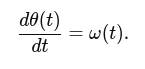
To obtain θ(t), you integrate the angular velocity over time:
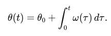
If you sample ω at discrete time steps tk = kΔt (where Δt is the sampling period), you can approximate the integral numerically. A simple numerical integration (Euler method) is:

Here, θk and ωk are the angle and angular velocity at the k-th time step.
From Linear Acceleration to Position
The position is related to acceleration by two integrations:
Acceleration to velocity:
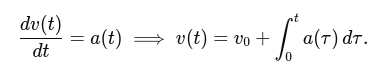
Velocity to position:
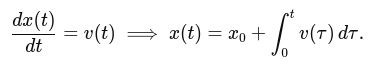
Combining these, we get:
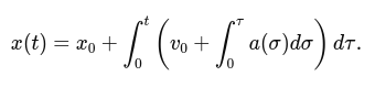
For discrete time steps, using Euler integration:
Update velocity:
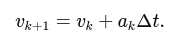
Update position:
Note that the velocity used to update the position can be the already updated velocity (vk+1) or the old one (vk), depending on your numerical integration choice. The simplest Euler method uses the old values:
But for clarity and consistency, you might update position using the updated velocity if you wish (this is a matter of integration scheme choice; either is acceptable for this tutorial).
Step-by-Step Example
Setup:
Assume a sampling frequency of fs = 100 Hz (Δt = 0.01s).
Suppose we have a constant angular velocity ω = 0.1 rad/s and a constant acceleration a = 0.2 m/s^2.
Initial orientation: θ0 = 0 rad.
Initial velocity: v0 = 0 m/s.
Initial position: x0 = 0 m.
Orientation Calculation:
θk+1 = θk + ωkΔt.
Since ωk = 0.1 rad/s is constant, after one step:

After 100 steps (1 second):

Position Calculation:
Velocity update:

After the first step:
Position update:

(Since initial velocity is zero, position doesn't change in the first iteration.)
Next step:
Practical Considerations
- Noise and Biases: Real IMU data is noisy. Integrating noisy data leads to drift. In practice, filtering (e.g., using a Kalman filter or complementary filter) is essential.
- Gravity Compensation: If you are working in 3D, you must subtract the gravity vector from the accelerometer reading to isolate the linear acceleration. In 1D, if your axis is aligned vertically, you must subtract out
g = 9.81 m/s^2. - Sampling Rate and Integration Method: We used a simple Euler method. More accurate integration schemes (e.g., trapezoidal, Runge-Kutta) can improve accuracy.
Example Code
import numpy as np
import matplotlib.pyplot as plt

# Simulation parameters
fs = 100.0              # sampling frequency (Hz)
dt = 1.0/fs             # time step
t_end = 5.0             # total duration (s)
t = np.arange(0, t_end, dt)

# Given sensor readings (for demonstration)
omega = 0.1 * np.ones_like(t)  # rad/s
a = 0.2 * np.ones_like(t)       # m/s^2

# Initial conditions
theta_0 = 0.0
x_0 = 0.0
v_0 = 0.0

# Allocate arrays for orientation, velocity, and position
theta = np.zeros_like(t)
v = np.zeros_like(t)
x = np.zeros_like(t)

theta[0] = theta_0
v[0] = v_0
x[0] = x_0

# Numerical integration
for k in range(len(t)-1):
    # Integrate orientation
    theta[k+1] = theta[k] + omega[k]*dt

    # Integrate velocity
    v[k+1] = v[k] + a[k]*dt

    # Integrate position
    x[k+1] = x[k] + v[k]*dt

# Plot results
plt.figure(figsize=(12,6))

plt.subplot(3,1,1)
plt.plot(t, theta, label='Orientation (rad)')
plt.xlabel('Time (s)')
plt.ylabel('Theta (rad)')
plt.title('Orientation from Angular Velocity')

plt.subplot(3,1,2)
plt.plot(t, v, label='Velocity (m/s)')
plt.xlabel('Time (s)')
plt.ylabel('Velocity (m/s)')
plt.title('Velocity from Acceleration')

plt.subplot(3,1,3)
plt.plot(t, x, label='Position (m)')
plt.xlabel('Time (s)')
plt.ylabel('Position (m)')
plt.title('Position from Acceleration')

plt.tight_layout()
plt.show()

Tip: Try to add some random noise to measured signals.
Advanced Topics (future robotics courses)
- Extend the logic to 3D, working with vectors and rotation representations (e.g., Euler angles, quaternions).
- Implement filtering techniques to handle noise (e.g., a complementary filter to fuse accelerometer and gyroscope data).
- Learn how to remove gravity from the accelerometer measurements in real-world scenarios.
- Implement full 3D orientation estimation with drift compensation (lin acc to estimate gravity direction, gyro for quick orientation updates).
Maze Escape
This short guide outlines a simple strategy for escaping a maze with a differential-drive robot using the right-hand rule (wall following). It is intentionally minimal and practical.
Idea
- Keep your right side close to a wall and keep moving forward.
- When you hit an opening on the right, turn right and follow the new corridor.
- If you reach a dead end, turn around and continue following the right wall.
This works in simply-connected mazes (no isolated loops). In general mazes with loops, it still explores systematically but may revisit areas.
Sensing Options
- Proximity sensors or bumpers (short range): detect walls and contacts.
- IR/ultrasonic rangefinders: measure distance to right/left/front walls.
- 2D LIDAR: robust wall detection with angles and distances.
Minimal Right-Hand Rule (pseudocode)
RIGHT = 1     # sensor index or side identifier
FRONT = 0

while True:
    right_clear = sense_opening(side=RIGHT)
    front_clear = sense_opening(side=FRONT)

    if right_clear:
        turn_right()
        drive_forward()
    elif front_clear:
        drive_forward()
    else:
        turn_left()  # or turn around if completely blocked
Practical Tips
- Maintain a small, roughly constant right-wall distance if you have distance sensors; a simple PD controller on lateral error improves stability.
- Use a minimum forward speed to avoid stalling, and cap turn rates for smooth motion.
- Debounce sensor changes and use timeouts to avoid oscillations at junctions.
Troubleshooting
- Robot gets stuck oscillating at corners: reduce speed, add a short delay after turns, and/or add hysteresis to “opening detected.”
- Loses the wall at gaps/doorways: keep moving forward briefly while searching for the wall again; if not found, slow down and rotate to reacquire.
- Drifts into walls: add a small proportional correction on measured right-wall distance.
Others
Linux
Installation
To install Ubuntu Linux, follow the official documentation: https://ubuntu.com/tutorials/install-ubuntu-desktop#1-overview
VirtualBox Installation (VB)
If you don’t have a spare machine for a clean Linux installation or cannot dual boot, consider installing Linux in a virtual machine.
VirtualBox is an example of a virtual machine hypervisor that allows you to run Linux on a different host OS.
Install VirtualBox following the instructions for your operating system:
- Windows and macOS: https://www.virtualbox.org/wiki/Downloads
- Linux: the process depends on your distribution and package manager. For Debian/Ubuntu:
- In a terminal:
sudo apt install virtualbox - Launch VirtualBox by running
virtualboxor from your applications menu.
- In a terminal:
To install Ubuntu inside the virtual machine, follow: https://ubuntu.com/tutorials/how-to-run-ubuntu-desktop-on-a-virtual-machine-using-virtualbox#1-overview
CLI (Command Line Interface)
Consider this chapter a quick guide for working with the Linux terminal.
You don’t need to memorize every command and parameter; be familiar with the basics and know how to look up usage when needed.
Helpful cheat sheet: https://assets.ubuntu.com/v1/2950553c-OpenStack%20cheat%20sheet%20-%20revised%20v3.pdf
Command
Explanation of function
Example usage ... Explanation
ls — list
Displays files and directories in the current location.
ls
ls -la      # lists all files, including hidden ones, with details
cd — change directory
Changes the current directory.
cd my_directory      # moves into the directory named "my_directory"
cd ~                 # goes to your home directory
cd ..                # moves up one directory level
cd /                 # goes to the filesystem root
cd ../my_folder      # up one level, then into "my_folder"
cd .                 # stays in the current directory ("." means current directory)
pwd — print working directory
Shows the current directory path.
pwd
mkdir — make directory
Creates a new directory.
mkdir my_folder # creates a directory named "my_folder"
cp — copy
Copies files.
cp source_file destination_file             # creates a copy of "source_file" named "destination_file"
cp ../secret.txt secret_folder/supersecret.txt  # copies "secret.txt" from the parent directory to "secret_folder" as "supersecret.txt"
mv — move (rename)
Originally moved files; today also commonly used to rename files.
mv old_name.txt new_name.html # renames "old_name.txt" to "new_name.html"
rm — remove
Deletes files or directories.
rm old_file.txt      # deletes the file "old_file.txt"
rm -r my_folder      # deletes a directory and its contents (recursive)
chmod — change mode
Changes file access permissions.
chmod 777 /dev/ttyUSB0 # grants all users access to USB port 0 (example)
sudo — run as administrator
Executes a command with administrator (root) privileges. Commonly used to modify system files.
sudo mkdir /etc/config      # creates a "config" directory in "/etc"
sudo rm -r /                # DANGEROUS: recursively deletes the root directory (destroys the system)
cat — Concatenate file(s) to standard output
Prints file contents to the terminal.
cat ~/my_config_file.txt
man — manual
Displays the manual for a program.
man ls
Linux Distributions
Linux refers to the operating system kernel, maintained by Linus Torvalds and community contributors.
Above the kernel is a layer of package management, desktop environments, and supporting software. A Linux “distribution” bundles these components and is provided by a specific organization or vendor.
Common distributions:
- Debian — Very widespread.
- Ubuntu — Based on Debian; popular for desktops.
- Linux Mint — Based on Ubuntu; Windows-like GUI.
- Raspberry Pi OS (formerly Raspbian) — Debian-based for Raspberry Pi.
- Arch Linux — For advanced users; highly customizable.
- Fedora — A popular alternative to Debian-based systems.
- elementary OS — Minimalist and fast; good for low-spec machines.
- …and many more.
Essential Programs
apt
Debian/Ubuntu package manager. Software is installed from trusted repositories.
Administrator privileges are required to install software.
Example: install Git
sudo apt update
sudo apt install git
nano
A simple text editor similar to Notepad.
- Ctrl+X — Exit (prompts to save changes)
vim
A powerful text editor with a steeper learning curve. It can be much faster than nano once learned. Consider a beginner tutorial before using.
If you open vim by accident, exit with Shift+Z+Z (hold Shift and press Z twice).
mc
Midnight Commander — a text-based file manager reminiscent of MS-DOS.
- F10 — Exit
curl
Command-line tool for transferring data over various protocols. Often used for HTTP requests or downloads.
wget
Downloads files from the internet. Example: download the latest WordPress release
wget https://wordpress.org/latest.zip
Final Words
If you’re new to Linux, don’t be afraid to experiment. Ideally, use a VirtualBox VM and create a snapshot/backup. If you break the system, restore the snapshot and continue working.
C++
Warmup Quiz
- What will be the output of the following code?
#include <iostream>
int main() {
    int x = 5;
    int* p = &x;
    *p = 10;
    std::cout << x << '\n';
    return 0;
}
-
What does the
constkeyword do when applied to a variable? -
What is the difference between
structandclassin C++? -
What is the purpose of a constructor in a class?
-
Explain the difference between a pointer and a reference.
-
What will be the output of the following code?
#include <iostream>
#include <vector>
int main() {
    std::vector<int> v = {1, 2, 3};
    for (auto it = v.begin(); it != v.end(); ++it) {
        std::cout << *it << " ";
    }
    return 0;
}
-
In your own words, explain what the Standard Template Library (STL) is.
-
What will be the output of the following code?
#include <iostream>
class Base {
public:
    virtual void print() {
        std::cout << "Base class\n";
    }
};

class Derived : public Base {
public:
    void print() override {
        std::cout << "Derived class\n";
    }
};

int main() {
    Base* b = new Derived();
    b->print();
    delete b;
    return 0;
}
-
Explain the difference between
std::array<T, N>andstd::vector<T>. -
Explain the output of the following lambda-based code.
#include <iostream>
int main() {
    int a = 10, b = 20;
    auto sum = [&]() -> int { return a + b; };
    b = 30;
    std::cout << sum() << '\n';
    return 0;
}
Revisiting Fundamentals
Functions and Pointers
Functions are the building blocks of C++ programs, and pointers are fundamental for memory management. Let’s revisit these concepts with an example.
#include <iostream>
void swap(int* a, int* b) {
    int temp = *a;
    *a = *b;
    *b = temp;
}

int main() {
    int x = 5, y = 10;
    std::cout << "Before swap: x = " << x << ", y = " << y << '\n';
    swap(&x, &y);
    std::cout << "After swap: x = " << x << ", y = " << y << '\n';
    return 0;
}
Discussion Points:
- What happens when you pass pointers versus values?
- When would you use references instead of pointers?
Object-Oriented Programming (OOP)
Object-oriented programming is key to structuring large projects in C++. Let’s review how classes and inheritance work.
#include <iostream>
#include <string>

class BankAccount {
private:
    std::string owner;
    double balance;

public:
    BankAccount(const std::string& owner, double balance)
        : owner(owner), balance(balance) {}

    void deposit(double amount) {
        balance += amount;
    }

    void withdraw(double amount) {
        if (amount <= balance)
            balance -= amount;
        else
            std::cout << "Insufficient funds!\n";
    }

    void display() const {
        std::cout << owner << "'s balance: $" << balance << '\n';
    }
};

int main() {
    BankAccount account("John Doe", 1000.0);
    account.display();
    account.deposit(500);
    account.withdraw(300);
    account.display();
    return 0;
}
Discussion Points:
- What is the purpose of the
privatekeyword? - How does the
constqualifier ensure safety indisplay()?
Modern C++ Features
Raw pointers are error-prone. Smart pointers, introduced in C++11, simplify memory management.
std::unique_ptr:
- Exclusive ownership: only one
std::unique_ptrcan point to a resource at a time.
#include <iostream>
#include <memory>
#include <string>

class MyClass {
public:
    explicit MyClass(std::string name) : name_{std::move(name)} { std::cout << "Constructor called " << name_ << std::endl; }
    ~MyClass() { std::cout << "Destructor called " << name_ << std::endl; }
private:
    std::string name_;
};

int main() {
    {   // Create a scope to demonstrate smart pointer behavior
        std::unique_ptr<MyClass> u_ptr = std::make_unique<MyClass>("unique");
        MyClass* raw_ptr = new MyClass("raw");
    }   // end of scope; u_ptr goes out of scope, destructor is called automatically
    // raw_ptr is not deleted, causing a potential memory leak

    return 0;
}
std::shared_ptr:
- Shared ownership: multiple
std::shared_ptrcan point to the same resource. - Reference counting: the resource is deleted when the last
std::shared_ptrgoes out of scope.
#include <iostream>
#include <memory>

class MyClass {
public:
    MyClass() { std::cout << "MyClass constructor\n"; }
    ~MyClass() { std::cout << "MyClass destructor\n"; }
};

int main() {
    std::shared_ptr<MyClass> sp1 = std::make_shared<MyClass>();
    std::cout << "Use count: " << sp1.use_count() << std::endl;

    {
        std::shared_ptr<MyClass> sp2 = sp1;
        std::cout << "Use count: " << sp1.use_count() << std::endl;
    }

    std::cout << "Use count: " << sp1.use_count() << std::endl;
    return 0;
}
std::weak_ptr
- Weak reference: does not affect the reference count of the shared resource.
- Doesn’t increase the reference count.
- Used to prevent circular references in shared ownership.
#include <iostream>
#include <memory>

class NodeB; // forward declaration

class NodeA {
public:
    std::shared_ptr<NodeB> strong_ptr; // Strong reference to NodeB
    std::weak_ptr<NodeB> weak_ptr;     // Weak reference to NodeB
    NodeA() { std::cout << "NodeA constructor\n"; }
    ~NodeA() { std::cout << "NodeA destructor\n"; }
};

class NodeB {
public:
    std::shared_ptr<NodeA> strong_ptr; // Strong reference to NodeA
    std::weak_ptr<NodeA> weak_ptr;     // Weak reference to NodeA
    NodeB() { std::cout << "NodeB constructor\n"; }
    ~NodeB() { std::cout << "NodeB destructor\n"; }
};

int main() {

    { // create scope
        std::cout << "Entering first scope..." << std::endl;
        // Create NodeA and NodeB, each referencing the other.
        auto a = std::make_shared<NodeA>();
        auto b = std::make_shared<NodeB>();
        a->strong_ptr = b; // NodeA has a strong reference to b
        b->strong_ptr = a; // NodeB has a strong reference to a
        std::cout << "Exiting first scope..." << std::endl;
    } // end scope

    // Here, a and b go out of scope, but each Node holds a strong pointer to the other.
    // Their reference counts never reach zero, so destructors are NOT called.
    // This leads to a memory leak because NodeA and NodeB remain alive, referencing each other.

    { // create new scope
        std::cout << "Entering second scope..." << std::endl;
        auto a = std::make_shared<NodeA>();
        auto b = std::make_shared<NodeB>();
        a->strong_ptr = b; // NodeA has a strong reference to b
        b->weak_ptr = a;   // NodeB has a weak reference to a
        std::cout << "Exiting second scope..." << std::endl;
    }

    return 0;
}
Discussion Points:
- What happens when the
std::unique_ptrgoes out of scope? - Compare
std::shared_ptrandstd::unique_ptr. - When should you use
std::weak_ptr? - Should we use raw pointers in modern C++? — Generally, no.
Functions as Objects
Lambda Functions
Lambda functions (also called lambda expressions) in C++ are unnamed (anonymous) functions that you can define inline. They were introduced in C++11 to make it easier to create small, concise functions, especially for use with the Standard Template Library (STL) algorithms or as callbacks. Unlike regular functions, they can capture variables from their surrounding scope. This is incredibly useful for passing context to a function on the fly.
Syntax:
[ capture_list ] ( parameter_list ) -> return_type {
    // function body
}
- capture_list: Which variables from the enclosing scope are available inside the lambda and how they are captured (by value, by reference, etc.).
- parameter_list: The parameters the lambda accepts (similar to a function’s parameter list).
- return_type: Often omitted because it can be deduced by the compiler, but can be specified explicitly using
-> return_type. - function body: The code that executes when the lambda is called.
Example of lambda function usage:
#include <iostream>
#include <vector>
#include <algorithm>

int main() {
    std::vector<int> nums = {5, 2, 8, 3, 1};

    std::sort(nums.begin(), nums.end(), [](int a, int b) { return a < b; });

    for (int num : nums) {
        std::cout << num << ' ';
    }
    return 0;
}
Discussion Points:
- How does the lambda function work in
std::sort? - When should you use lambdas over named functions?
#include <iostream>
#include <vector>
#include <algorithm>

int main() {
    std::vector<int> values = {1, 2, 3, 4, 5};
    int offset = 10;

    auto printValue = [](int val) {
        std::cout << val << " ";
    };

    // Capture everything by value (copy)
    std::for_each(values.begin(), values.end(), [=](int val) {
        // Modifies a copy of 'val', not the element itself
        int tmp = val + offset;
        (void)tmp; // suppress unused-variable warning in this snippet
        // offset += 1; // error: 'offset' cannot be modified; use [=]() mutable { ... } to allow modification
    });
    std::for_each(values.begin(), values.end(), printValue);

    // Capture everything by reference
    std::for_each(values.begin(), values.end(), [&](int& val) {
        val += offset;   // modifies 'val' directly in the vector via reference
        offset += 1;
    });
    std::for_each(values.begin(), values.end(), printValue);

    std::cout << std::endl;
    return 0;
}
std::function
A flexible, type-erased wrapper that can store function pointers, lambdas, or functor objects. It is part of the C++ Standard Library and is useful for creating callbacks or function objects that can be passed around like variables.
#include <iostream>
#include <functional>

int sum(int a, int b) {
    return a + b;
}

int main() {
    std::function<int(int, int)> func1 = sum;
    std::function<int(int, int)> func2 = [](int a, int b) { return a * b; };

    std::cout << "sum(3, 4): " << func1(3, 4) << std::endl;
    std::cout << "multiply(3, 4): " << func2(3, 4) << std::endl;

    return 0;
}
Coding Challenge
Task: Create a simple program to manage student records, including adding and displaying students.
- Use a
Studentclass with properties for name, age, and grades. - Store students in a
std::vector. - Implement a menu-driven program for user interaction.
#include <iostream>
#include <vector>
#include <string>

class Student {
private:
    std::string name;
    int age;
    std::vector<int> grades;

public:
    Student(const std::string& name, int age) : name(name), age(age) {}

    void addGrade(int grade) {
        grades.push_back(grade);
    }

    void display() const {
        std::cout << "Name: " << name << ", Age: " << age << ", Grades: ";
        for (int grade : grades) {
            std::cout << grade << ' ';
        }
        std::cout << '\n';
    }
};

int main() {
    std::vector<Student> students;

    // Add menu-driven functionality here
    return 0;
}
CMake
CMake is a cross-platform build system generator. You describe your project in plain text files named CMakeLists.txt, and CMake generates native build files for your platform, such as Makefiles (Unix), Ninja files, or Visual Studio solutions (Windows).
Key ideas:
- Target-based: Modern CMake focuses on targets. You create targets (executables or libraries) and attach properties to them (include directories, compile features, linked libraries, compile definitions, etc.). Most modern commands start with
target_...and take the target name as the first argument. - Dependency management:
find_package()locates external dependencies (optionally checking versions/components), and you link them to your targets.
Basic example
A small C++ project structure:
MyProject/
  include/
    movement/
      move.hpp
      turn.hpp
    talk.hpp
  src/
    movement/
      move.cpp
      turn.cpp
    talk.cpp
    main.cpp
  CMakeLists.txt
Minimal CMakeLists.txt:
cmake_minimum_required(VERSION 3.15)

project(MyProject VERSION 1.0
        DESCRIPTION "Very nice project"
        LANGUAGES CXX)

# Prefer target-specific settings in modern CMake. If you want a global default:
set(CMAKE_CXX_STANDARD 17)
set(CMAKE_CXX_STANDARD_REQUIRED ON)
set(CMAKE_CXX_EXTENSIONS OFF)

add_executable(MyProject
  src/main.cpp
  src/talk.cpp
  src/movement/move.cpp
  src/movement/turn.cpp
)

# Tell the target where to find headers under include/
# Use PUBLIC to propagate include paths to dependents (if this were a library).
target_include_directories(MyProject PUBLIC ${CMAKE_SOURCE_DIR}/include)
Explanation:
cmake_minimum_required(VERSION 3.15)sets the minimum CMake version that can process this project.project(...)defines project metadata. It does not implicitly create a target; you still needadd_executable()oradd_library().- C++ standard: Using
set(CMAKE_CXX_STANDARD 17)defines a project-wide default. Alternatively, you can set features per-target withtarget_compile_features(MyProject PUBLIC cxx_std_17). add_executable(MyProject ...)declares the build target and lists its source files. Header files need not be listed; they are discovered by the compiler via include paths.target_include_directories(MyProject PUBLIC include)associates include paths with the target. Visibility keywords: PRIVATE (only this target), PUBLIC (this target and its dependents), INTERFACE (only dependents).
Build the example
Common out-of-source build workflow:
# from the project root (MyProject/)
cmake -S . -B build -DCMAKE_BUILD_TYPE=Release   # configure
cmake --build build --config Release             # build
./build/MyProject                                # run the executable (Unix-like)
For debugging builds (e.g., with gdb):
cmake -S . -B build -DCMAKE_BUILD_TYPE=Debug
cmake --build build --config Debug
Note: On multi-config generators (e.g., Visual Studio), specify --config Debug when building and running.
Including libraries
As a simple example with OpenCV. This assumes OpenCV is installed and discoverable by CMake.
cmake_minimum_required(VERSION 3.15)
project(MyProject LANGUAGES CXX)

# Optionally request specific components and/or versions
find_package(OpenCV REQUIRED COMPONENTS core imgproc highgui)

add_executable(MyProject main.cpp)

# Link libraries target-based; include paths typically come via the imported target
# but if you rely on variables, you can still use them.
target_link_libraries(MyProject PRIVATE ${OpenCV_LIBS})
# If needed (older packages), add include dirs explicitly
if(OpenCV_INCLUDE_DIRS)
  target_include_directories(MyProject PRIVATE ${OpenCV_INCLUDE_DIRS})
endif()
Prefer packages that provide imported CMake targets (e.g., OpenCV::opencv_core, etc.) and link to those instead of raw variables when available:
# Example when imported targets are available
# target_link_libraries(MyProject PRIVATE opencv_core opencv_imgproc opencv_highgui)
Common target commands (cheat sheet)
add_executable(name sources...)/add_library(name [STATIC|SHARED|INTERFACE] sources...)target_link_libraries(tgt PRIVATE|PUBLIC|INTERFACE libs...)target_include_directories(tgt PRIVATE|PUBLIC|INTERFACE dirs...)target_compile_definitions(tgt PRIVATE|PUBLIC|INTERFACE MACRO=VALUE ...)target_compile_features(tgt PRIVATE|PUBLIC cxx_std_17 ...)
Resources
- Modern CMake guide: https://cliutils.gitlab.io/modern-cmake/README.html
- CMake official documentation: https://cmake.org/cmake/help/latest/
Git - Version Control System
Git is a distributed system for versioning and managing backups of source code. However, Git also works well for versioning any kind of text. The primary motivation for teaching Git in this course is the fact that Git is the most widely used version control system in the commercial sphere today, and there is a vast array of Git-based online version control services available on the web.
Basic Terminology
Let’s define some basic terms to ensure we’re on the same page.
Repository (repo)
A set of versioned files and records of their history. If the repository is stored on our computer, it is called a local repository (local repo). If it is stored on another machine, it is referred to as a remote repository (remote repo).
Cloning
Downloading a repository from a remote repo. Cloning occurs when the repository does not yet exist on the local machine.
Snapshot
The state of the repository at a specific point in its history.
Diff
The difference between two snapshots, i.e., the changes in the state of versioned files.
Commit
A record that contains a reference to the previous and next snapshot, as well as the diff between them. Each commit has a unique 20-byte hash that identifies it within the repository.
Push
Uploading new commits to the remote repository.
Fetch
Downloading commits from a remote repo to the local machine. Fetching is done when the local repository is already cloned but does not have the latest commits downloaded.
Branch
A sequence of interconnected commits. By default, every repository has one branch (typically named "master" or "main"). If multiple features are being developed simultaneously, these developments can be divided into separate branches and merged back into the main branch once the feature is complete.
How Git Works
The primary function of Git is versioning text files. It is important to note that Git is NOT suitable for versioning binary files. When developing a program and using Git for version control, you should always version source code only, never compiled executable files (binaries).
Git also enables highly efficient collaboration among multiple people working on the same project (repository). Developers can work together or individually on separate branches. However, a key rule is that two people must not overwrite the same line of code in two different commits, as this will cause a conflict. A general recommendation is that two people should avoid modifying the same file.
Unlike SVN, Git is a decentralized system. This means there is no superior, central repository or server. All repositories have the same functionality, can maintain the full history of the project, and can seamlessly communicate with all other clones. In practice, however, there is often a repository that acts as a central point for sharing commits between developers, commonly referred to as "origin".
It is important to note that any repository can download the complete history from the origin. In the event of an origin failure, no data is lost, as each developer has a complete copy of the repository on their computer.
Typical Workflow with Git:
- A repository is created on the server for the project.
- Developers clone the repository to their local machines. From their perspective, the server is referred to as "origin".
- Developers work on their local machines, creating code and committing changes.
- At the end of the day, each developer pushes their daily commits to the origin.
- The next morning, each developer fetches the commits from their colleagues made the previous day.
Installing Git on Linux
If you are using a Debian-based distribution, Git can be installed using the following commands:
sudo apt install git
or
sudo snap install git
Command Overview
git init
Initializes a repository, turning a regular folder in the file system into a repository. A repository differs from a regular folder because it contains a hidden .git folder that stores the repository's history.
git init # Initializes a repository
git add
Adds changes made since the last commit to the index. The index is a staging area where changes are prepared for the next commit. This allows selective inclusion of changes in a commit.
git add myfile.txt     # Adds changes made to 'myfile.txt' to the index
git add .              # Adds all current changes to the index
git commit
Creates a new commit derived from the last commit in the current branch. Includes changes (diffs) staged in the index.
git commit -m "Commit message" # Creates a new commit in the current branch
git checkout
Switches between snapshots.
git checkout .          # Reverts the branch to the last commit, discarding all changes
git checkout abcdef     # Switches to the state after commit 'abcdef'
git checkout master     # Switches to the last available commit in the 'master' branch
git clone
Creates a local clone of a remote repository. No need to initialize with git init, as repository metadata is automatically downloaded along with the content.
git clone https://remote_repo_address.git # Clones the repository to the local machine
git remote
Manages connections to remote repositories.
git remote -v                                            # Lists the configuration of remote repositories
git remote add origin https://remote_repo_address.git    # Adds a remote alias named 'origin'
git remote remove origin                                 # Removes the 'origin' alias
git push
Uploads new commits from the local repository to the remote repository.
git push origin master # Pushes new commits from the 'master' branch to the remote repository
git fetch
Downloads commits from the remote repository to the local repository. These commits are not automatically merged into the current branch.
git fetch origin           # Fetches all new commits from all branches of the 'origin'
git fetch origin master    # Fetches new commits for the 'master' branch from the 'origin'
git merge
Creates a new commit in the current branch by merging changes from another branch, combining all their changes.
git merge cool_branch # Merges the changes from 'cool_branch' into the current branch
git pull
Combines git fetch and git merge. Commonly used to pull changes from a remote repository. It fetches commits from the remote repository and then merges them into the current branch.
git pull origin master # Fetches and merges commits from 'master' branch of 'origin'
git diff
Displays the difference between two snapshots (commits).
git diff abcdef 012345 # Shows the difference between commits 'abcdef' and '012345'
git status
Shows the current state of changes since the last commit, including changes already staged in the index.
git status # Displays the current state of changes
git log
Displays a chronological history of commits along with their metadata (timestamp, commit message, hash, etc.).
git log # Displays the history of the current branch
git stash
Saves and retrieves changes to/from a stack. Useful when you realize you are working on the wrong branch. Changes can be stashed, allowing you to switch branches and reapply the changes later.
git stash        # Saves changes to the stack and reverts the branch to its state after the last commit
git stash pop    # Retrieves changes from the stack and applies them to the current state
Exercise
Basic Operations
- Create a repository.
- Create two text files in the repository and write a few lines in each.
- Add the changes to the index and then commit them.
- Edit one of the files and commit the changes.
- Edit the second file and commit the changes.
- Create an account on GitHub and create a new repository there.
- Add the remote repository as "origin" to your local repository and push the changes to the origin.
- Verify the repository's contents in the GitHub web interface.
- On another location on your computer, or on a different computer, clone the repository you just pushed.
- In the new clone, make a change, commit it, and push it to the origin.
- In the original folder, pull the new commits from the origin.
- Use the
git logcommand to view the commit history.
Conflict
An example of what happens when two developers change the same code.
- Following the steps from the previous exercise, create two copies of the repository on the same computer or two different computers, both with the same origin on GitHub.
- In the first clone, modify a specific line in a file, commit the change, and push it to the origin.
- In the second clone, modify the same line, commit the change, and try to push (this will result in an error).
- A conflict has been created. Two conflicting changes occurred at the same point in the repository's branch history.
- Resolve the conflict by pulling from the origin in the second clone where the push failed.
- Open the file containing the conflict. The conflict will be marked with special syntax:
Choose the desired version, remove the conflict markers, and save the file. The conflict is now resolved.<<<<<<< local_change ======= change_from_origin >>>>>>> - Run the
git commitcommand without additional parameters to commit the resolved conflict. An automatic commit message will indicate that this is a conflict resolution. - Push the new commit to the origin, then pull it into the original repository.
- Use the
git logcommand to view the commit history.
Other Resources
- Git Cheat Sheet: https://education.github.com/git-cheat-sheet-education.pdf
- Atlassian Git Tutorials: https://www.atlassian.com/git/tutorials
- Official Git Documentation: https://git-scm.com/doc
- Oh Shit, Git!? A helpful guide: https://ohshitgit.com/
CLion
CLion is a JetBrains IDE for writing, building, running, and debugging C/C++ code. It provides an intuitive UI, modern tooling, and tight integration with CMake and version control systems like Git.
This guide explains how to use CLion for the BPC-PRP course. It covers installation, creating a simple “Hello, World!” program, and getting familiar with the IDE layout. Screenshots are from CLion 2024.3.3; newer versions may look slightly different.
CLion Installation
You can install CLion in two ways:
- Using Snap (Linux):
sudo snap install clion --classic - Download from JetBrains: https://www.jetbrains.com/clion/
Students can use the full version for free while studying. Request a student license here: https://www.jetbrains.com/community/education/
Hello World Project
Let’s create a simple Hello World project to learn how to create a project and run it locally.
When you open CLion, the Welcome screen lists your recent projects. Click “New Project”.

After clicking “New Project”, a dialog appears where you configure the project. Choose the project location and the C++ standard (use C++17 for this course).

After clicking “Create”, CLion opens the IDE where you can start working.
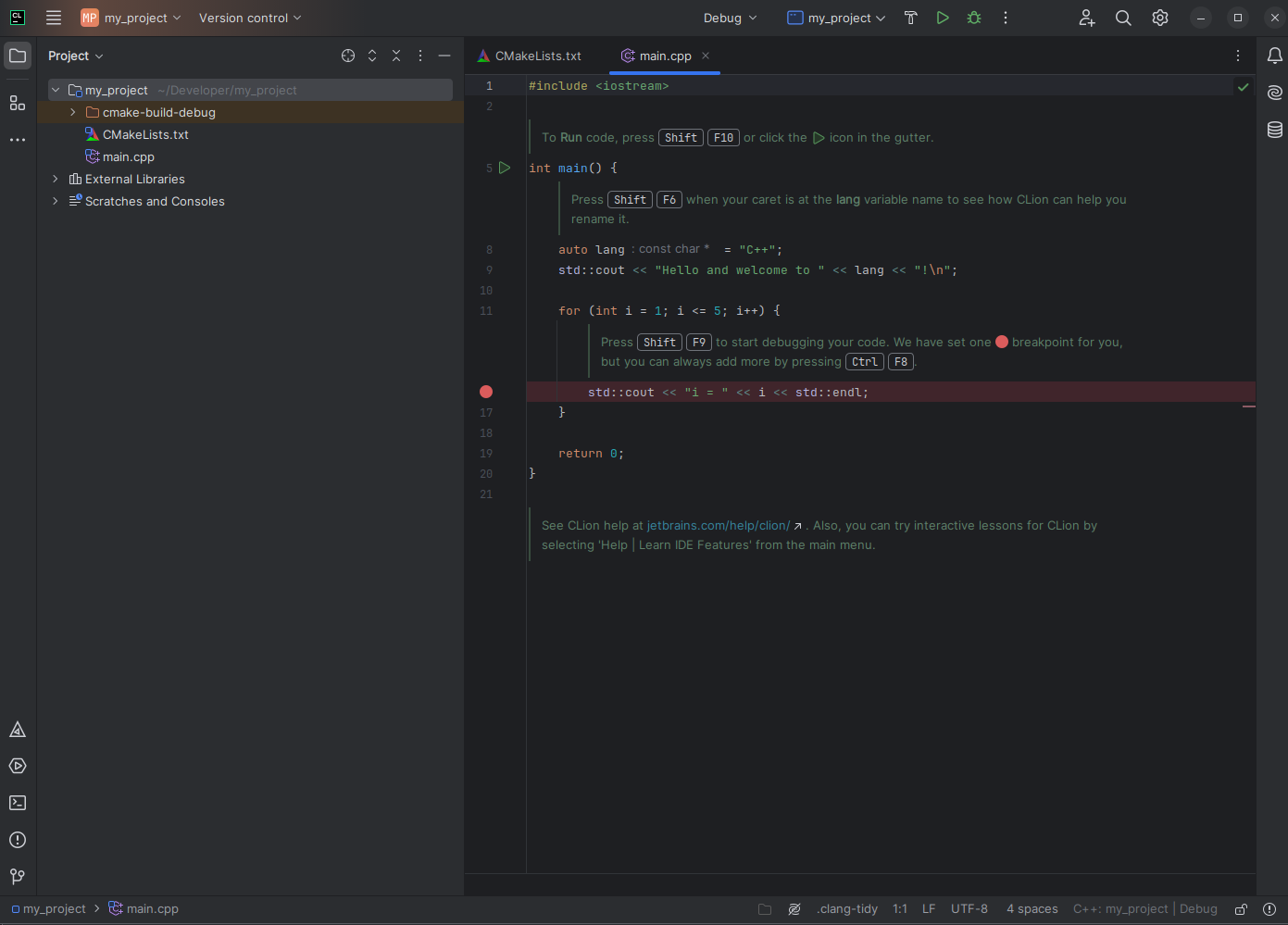
Key areas of the UI:
- Left: Project tool window (project files)
- Center: Editor (source code)
- Top toolbar: Build configuration (Debug/Release), target selector, and Build/Run/Debug buttons
- Bottom tool windows: CMake, Services, Terminal, Problems, Version Control
When your program runs, the Run tool window shows the output. This is where you’ll see messages like “Hello, World!” and any runtime errors to help with debugging.
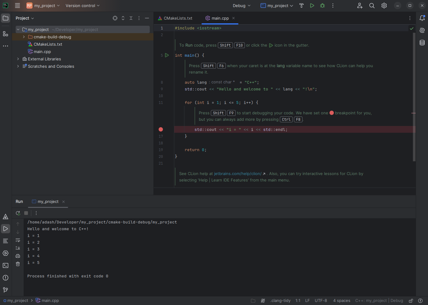
When you start a debug session, the Debug tool window and controls appear.
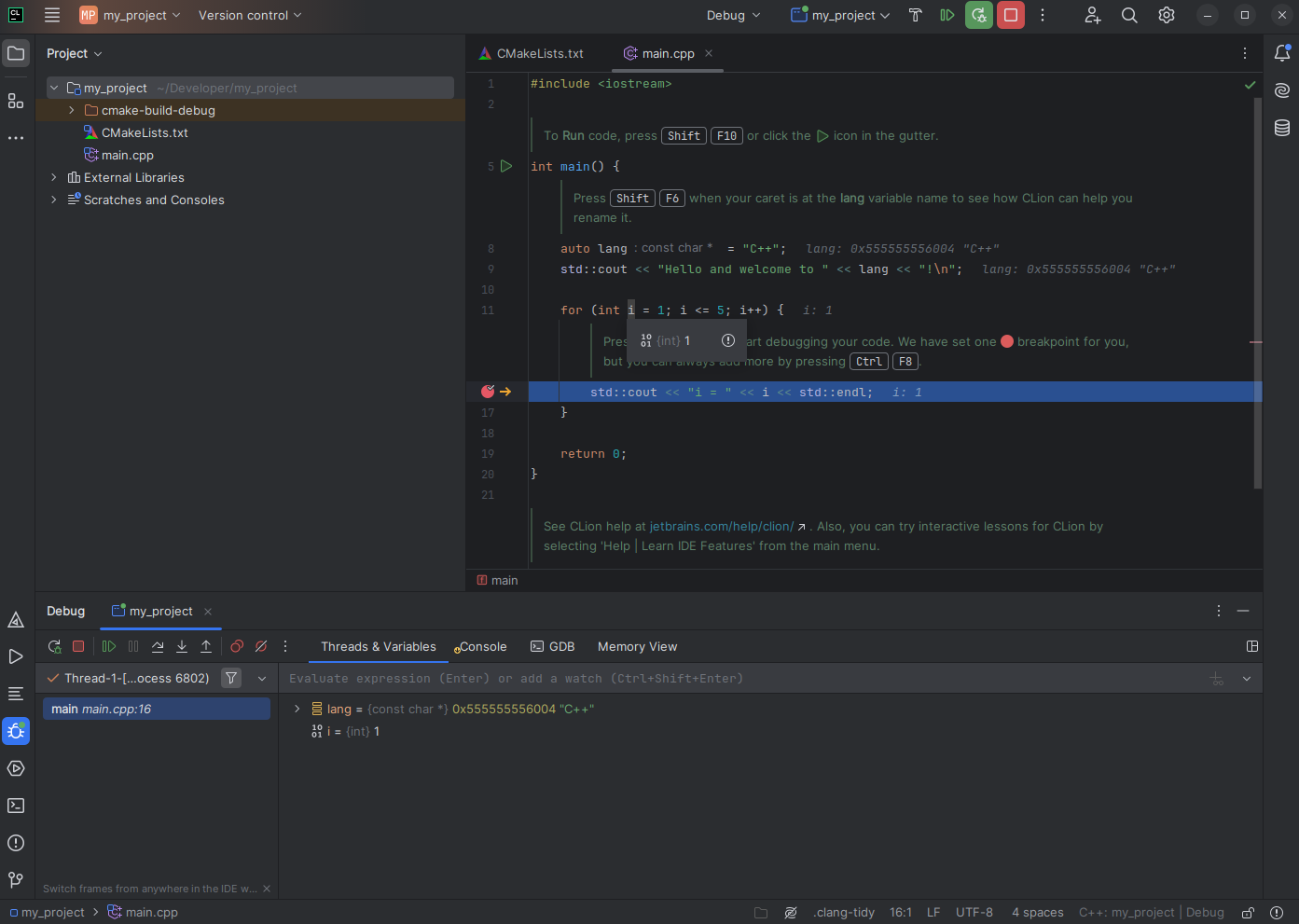
Integrated Tutorial
Recent CLion versions include an onboarding tutorial. Follow it to learn more about navigation, refactoring, debugging, and testing.
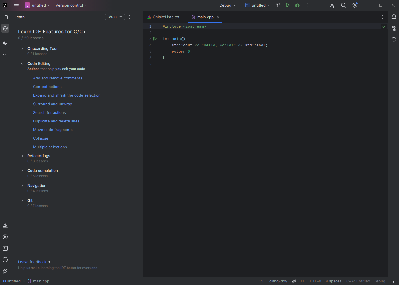
Multithreading
Motivation
Why use multiple threads?
- Modern CPUs have multiple cores; using multiple threads can improve performance by performing tasks in parallel.
- Some tasks, like handling multiple network connections, benefit from concurrent operations to remain responsive.
Key Concepts
- Concurrency vs. Parallelism:
- Concurrency is the composition of independently executing processes or threads.
- Parallelism is the simultaneous execution of (possibly related) computations, using multiple physical CPU cores.
- Threads: A thread is the smallest sequence of programmed instructions that can be managed independently by a scheduler.
Risks & Challenges of Multithreading
- Data Races: Two or more threads access a shared variable without proper synchronization, and at least one thread writes to the variable.
- Deadlocks: Two or more threads are blocked forever, each waiting for the other to release a resource.
- Race Conditions: A program’s outcome depends on the sequence of events or timings of threads.
- Complexity: Debugging and reasoning about concurrent programs is generally harder than single-threaded ones.
Basic Thread Creation and Management
The <thread> Header
Modern C++ (C++11 and above) provides a standard way to create and manage threads through the <thread> header.
// Example 1: Creating a Simple Thread
#include <iostream>
#include <thread>

void helloFunction() {
    std::cout << "Hello from thread!\n";
}

int main() {
    std::thread t(helloFunction); // Create a thread running helloFunction
    t.join();                     // Wait for the thread to finish
    std::cout << "Hello from main!\n";
    return 0;
}
Explanation:
std::thread t(helloFunction);creates a new thread that executeshelloFunction.t.join();ensures the main thread waits untiltfinishes.- If you omit
t.join(), the program may exit before the thread finishes, or you must callt.detach()if you intend the thread to run independently.
Lambda Functions with Threads
Instead of passing a function pointer, you can also pass a lambda:
// Example 2: Using a Lambda
#include <iostream>
#include <thread>

int main() {
    std::thread t([](){
        std::cout << "Hello from a lambda thread!\n";
    });

    t.join();
    std::cout << "Hello from main!\n";
    return 0;
}
Passing Arguments to Threads
You can pass arguments to the thread function by specifying them after the callable:
// Example 3: Passing Arguments
#include <iostream>
#include <thread>

void printValue(int x) {
    std::cout << "Value: " << x << "\n";
}

int main() {
    int num = 42;
    std::thread t(printValue, num);
    t.join();
    return 0;
}
Detaching Threads
t.detach()makes the thread run independently; the main thread does not wait for it.- Use with caution: A detached thread can lead to tricky bugs if you rely on shared data in it.
Synchronization Mechanisms
Mutex and Lock Guards
To avoid data races, you typically protect shared data with a mutex. Only one thread can lock a mutex at a time.
// Example 4: Using std::mutex and std::lock_guard
#include <iostream>
#include <thread>
#include <mutex>
#include <vector>

std::mutex m;
int sharedCounter = 0;

void increment(int iterations) {
    for(int i = 0; i < iterations; ++i) {
        // Lock the mutex before modifying shared resource
        std::lock_guard<std::mutex> lock(m);
        ++sharedCounter;
    }
}

int main() {
    std::vector<std::thread> threads;
    for(int i = 0; i < 5; ++i) {
        threads.emplace_back(increment, 10000);
    }

    for(auto& t : threads) {
        t.join();
    }

    std::cout << "Final value of sharedCounter: " << sharedCounter << "\n";
    return 0;
}
Important Points:
std::lock_guard<std::mutex>automatically locks the mutex upon creation and unlocks it when it goes out of scope.- This prevents forgetting to unlock, especially in the presence of exceptions or multiple return statements.
Unique Lock
std::unique_lock<std::mutex> is more flexible than std::lock_guard, allowing you to lock/unlock explicitly.
Condition Variables
- Condition variables allow threads to wait (block) until they are notified that some condition is true.
- They typically work with a mutex to ensure correct data access.
// Example 5: Producer-Consumer with Condition Variables
#include <iostream>
#include <thread>
#include <mutex>
#include <condition_variable>
#include <queue>
#include <chrono>

std::mutex mtx;
std::condition_variable cv;
std::queue<int> dataQueue;
bool finished = false;

void producer() {
    for(int i = 1; i <= 5; ++i) {
        {
            std::lock_guard<std::mutex> lock(mtx);
            dataQueue.push(i);
            std::cout << "Produced: " << i << "\n";
        }
        cv.notify_one(); // Notify one waiting thread
        std::this_thread::sleep_for(std::chrono::milliseconds(100));
    }

    // Signal that production is finished
    {
        std::lock_guard<std::mutex> lock(mtx);
        finished = true;
    }
    cv.notify_all();
}

void consumer() {
    while(true) {
        std::unique_lock<std::mutex> lock(mtx);
        cv.wait(lock, []{ return !dataQueue.empty() || finished; });
        if(!dataQueue.empty()) {
            int value = dataQueue.front();
            dataQueue.pop();
            std::cout << "Consumed: " << value << "\n";
        }
        else if(finished) {
            break; // No more data
        }
    }
}

int main() {
    std::thread prod(producer);
    std::thread cons(consumer);

    prod.join();
    cons.join();

    return 0;
}
Explanation:
- The producer thread pushes data to
dataQueueand notifies the consumer. - The consumer thread waits (
cv.wait) until it is notified that either new data is available or production is finished. cv.wait(lock, condition)atomically unlocks the mutex and sleeps untilconditionis true, then locks the mutex again before returning.
Atomic Operations
For simple operations like incrementing a counter, you can use std::atomic instead of a mutex:
#include <iostream>
#include <thread>
#include <atomic>
#include <vector>

std::atomic<int> sharedCounter(0);

void increment(int iterations) {
    for(int i = 0; i < iterations; ++i) {
        ++sharedCounter;
    }
}

int main() {
    const int threadCount = 5;
    std::vector<std::thread> threads;

    for(int i = 0; i < threadCount; ++i) {
        threads.emplace_back(increment, 10000);
    }

    for(auto& t : threads) {
        t.join();
    }

    std::cout << "Final Counter: " << sharedCounter.load() << "\n";
    return 0;
}
Note: Atomic operations are typically more efficient than locking but only suitable for simple scenarios (increment, bitwise operations, etc.).
Practical Examples and Exercise Ideas
Summation of Large Array in Parallel
One common pattern is to split a task into chunks that multiple threads work on.
#include <iostream>
#include <thread>
#include <vector>
#include <numeric>

void partialSum(const std::vector<int>& data, int start, int end, long long& result) {
    long long sum = 0;
    for(int i = start; i < end; ++i) {
        sum += data[i];
    }
    result = sum;
}

int main() {
    // Example data
    std::vector<int> data(1000000, 1); // 1 million elements of value 1

    long long result1 = 0, result2 = 0;
    int mid = data.size() / 2;

    // Create 2 threads to handle half the data each
    std::thread t1(partialSum, std::cref(data), 0, mid, std::ref(result1));
    std::thread t2(partialSum, std::cref(data), mid, data.size(), std::ref(result2));

    t1.join();
    t2.join();

    long long total = result1 + result2;
    std::cout << "Total sum: " << total << "\n";
    return 0;
}
Exercise: Extend the Summation
- Modify the code to use four threads instead of two.
- Compare performance for different numbers of threads and array sizes.
- Explore usage of std::mutex or
std::atomic<long long>if you want to accumulate into a single variable, but be mindful of performance overheads.
Exercise: Calculate Pi Using Multiple Threads
- Create multiple threads to estimate π by generating random points in a square and checking how many fall within the unit circle (Monte Carlo method).
- Each thread returns the count of points inside the circle; combine results in the main thread and compute the approximation of π.
- Compare performance with different thread counts.
Tips and Best Practices
-
Limit shared data
- Minimize the portion of code that needs synchronization to reduce contention.
-
Avoid excessive locking
- Use finer-grained locks or lock-free structures where applicable, but only if you fully understand the concurrency implications.
-
Use high-level concurrency abstractions if possible
- For example, C++17’s std::async and std::future or higher-level frameworks can simplify concurrency.
-
Always check for data races
- Tools like ThreadSanitizer can help detect concurrency issues.
-
Understand memory model
- C++ has a well-defined memory model for atomic operations and synchronization.
Resources
- C++ reference for threads: https://en.cppreference.com/w/cpp/thread
- C++ reference for mutexes and locks: https://en.cppreference.com/w/cpp/thread/mutex
- Condition variables: https://en.cppreference.com/w/cpp/thread/condition_variable
- Atomics and memory order: https://en.cppreference.com/w/cpp/atomic
- ThreadSanitizer (data race detector): https://github.com/google/sanitizers/wiki/ThreadSanitizer
Coordinate System
Understanding coordinate systems is essential for robotics, computer vision, and navigation. Coordinates let us describe where things are and how they are oriented in space. This chapter summarizes the most useful concepts and conventions you will meet in practice.
Frames, Axes, and Handedness
- Frame (coordinate frame): A local reference defined by an origin and three perpendicular axes (x, y, z). In 2D, you have two axes (x, y).
- Global vs. local: A global frame is a common reference for the whole scene (e.g., “map”). Local frames are attached to moving objects (e.g., “base_link” on a robot, “camera_link” on a camera).
- Handedness: The orientation of axes can be right‑handed or left‑handed. Most robotics software (ROS, linear algebra libraries) uses a right‑handed system.
- Right‑hand rule: Point index finger along +x, middle finger along +y, then the thumb gives +z.
Why it matters: Mixing left‑ and right‑handed systems or unclear axis labels causes mirrored motions, flipped images, and hard‑to‑debug sign errors.
2D vs. 3D
- 2D pose: (x, y, θ), where θ is heading/yaw about z.
- 3D pose: position (x, y, z) + orientation (rotation in 3D).
- Units: Use meters for distances and radians for angles unless otherwise documented. Be explicit.
Orientations in 3D
There are several equivalent ways to represent 3D rotation. Choose the one that fits your computations and interfaces.
- Euler angles (roll, pitch, yaw): Rotations about axes (commonly x, y, z). Easy to read; prone to gimbal lock and ambiguity (intrinsic vs. extrinsic, order matters: XYZ ≠ ZYX). Good for UI or logs, not for core math.
- Axis–angle: A unit axis vector â and an angle θ describe a single rotation about â. Compact and geometric.
- Rotation matrix R (3×3): Orthogonal matrix with det(R)=+1. Converts vectors between frames: v_B = R_AB · v_A (vector expressed in frame A to frame B). Great for composition; expensive to store many of them.
- Quaternion q = [w, x, y, z]: A unit quaternion encodes rotation without gimbal lock and composes efficiently. Preferred for interpolation and filtering.
Tip: Store orientation as a quaternion internally; convert to Euler only when needed for display.
Homogeneous Coordinates and Transforms
To represent position and orientation together, we use a 4×4 homogeneous transform T:
- Form: T = [ R t; 0 0 0 1 ], where R is 3×3 rotation and t is 3×1 translation.
- Applying a transform: In homogeneous coordinates p' = T · p, with p = [x, y, z, 1]^T.
- Composition: T_AC = T_AB · T_BC. Note the order: matrix multiplication is not commutative.
- Inverse: T_AB⁻¹ = [ Rᵀ −Rᵀ t; 0 0 0 1 ]. Use it to “go back” from B to A.
Interpretation: T_AB “takes” coordinates of a point expressed in frame B and returns coordinates expressed in frame A.
Composing and Chaining Frames (TF)
In robotics you often maintain a tree of frames (a “TF tree” in ROS terminology). Examples: map → odom → base_link → sensor frames.
- Composition rule: To express something in a different frame, multiply along the path in the correct order.
- Static vs. dynamic transforms: Some transforms are constant (sensor mounting), others change over time (robot motion). Time stamps matter when synchronizing sensors.
- Visualization: Tools like RViz2 can display axes for frames and arrows for transforms, helping you verify conventions early.
Common Frames in Robotics (ROS conventions)
ROS REP‑103 defines standard frames and axis directions (right‑handed, meters, radians):
- map: A world‑fixed frame; global, not required to be continuous.
- odom: A world‑fixed frame with continuous, drift‑accumulating motion estimate (no jumps).
- base_link: The robot body frame; usually at the robot’s geometric center on the ground plane.
- camera_link / camera_optical_frame: Camera frames; optical frame typically has +z forward (optical axis), +x right, +y down in ROS.
- imu_link, laser, wheel frames, etc., attached as children of base_link.
Always document where the origin is and how axes are oriented for each sensor. This makes extrinsic calibration reproducible.
Conventions and Best Practices
- Be explicit about units (m, rad) and handedness (right‑hand).
- Name frames consistently and publish a TF tree that matches your documentation.
- Keep transforms orthonormal: re‑normalize quaternions; ensure RᵀR ≈ I.
- Use consistent rotation order if using Euler angles; document it (e.g., XYZ intrinsic).
- Prefer quaternions for computation and interpolation; convert to Euler only for human‑readable outputs.
- Validate with visualization; a simple mistake (e.g., swapped axes) is obvious in RViz2.
Typical Pitfalls
- Degrees vs. radians: Many libraries expect radians; mixing them leads to large errors.
- Gimbal lock with Euler angles: Avoid for continuous orientation tracking.
- Flipped camera axes: Image coordinates (u, v) vs. camera optical frames can differ; check your library’s convention.
- Frame direction confusion: Clarify whether T_AB maps B→A or A→B. Name accordingly (read subscripts left‑to‑right for mapping direction).
- Non‑commutativity: R1·R2 ≠ R2·R1. Keep multiplication order straight.
Quick Cheat Sheet
- Right‑hand rule: x × y = z.
- Transform a point: p_A = T_AB · p_B.
- Compose transforms: T_AC = T_AB · T_BC.
- Inverse transform: T_BA = T_AB⁻¹ = [ Rᵀ −Rᵀ t; 0 0 0 1 ].
- Quaternion normalization: q ← q / ||q|| before use.
- From yaw (2D): R(θ) = [[cosθ, −sinθ],[sinθ, cosθ]].
Further Reading
- ROS REP‑103 (Standard Units of Measure and Coordinate Conventions): https://www.ros.org/reps/rep-0103.html
- A gentle quaternion primer (Eigen): https://eigen.tuxfamily.org/dox/classEigen_1_1Quaternion.html
- 3D Rotations, matrices, and quaternions (Wikipedia overview): https://en.wikipedia.org/wiki/Rotation_formalisms_in_three_dimensions
- tf2 tutorials (ROS2): https://docs.ros.org/en/foxy/Tutorials/tf2.html
- RViz2 basics: see “9_rviz2_visualizations.md” in this repository.
Communication Buses
This chapter summarizes four common serial buses used in embedded systems and robotics: UART, I2C, SPI, and CAN. For each, you’ll find the wiring, what problem it solves, typical speeds, and practical tips.
UART
A UART (Universal Asynchronous Receiver/Transmitter) sends and receives serial data one bit at a time over two data lines without a shared clock.
UART topology:

Key characteristics:
- Asynchronous: No clock line. Both ends must agree on the baud rate (bits per second).
- Signals: TX (transmit), RX (receive). Optional flow control lines RTS/CTS may be present.
- Frame format: start bit, 5–9 data bits (commonly 8), optional parity (even/odd/none), and one or two stop bits. Example: 8N1 = 8 data bits, no parity, 1 stop bit.
- Voltage levels: Commonly TTL/CMOS (e.g., 3.3 V or 5 V) on microcontrollers; classic RS‑232 levels are higher and inverted and require a level shifter (e.g., MAX232).
- Typical speeds: 9,600; 57,600; 115,200 baud; many MCUs support higher.
With UART, reliable communication requires matching configuration on both ends (baud rate, data bits, parity, stop bits). Parity can detect single‑bit errors but not correct them.
UART timing:
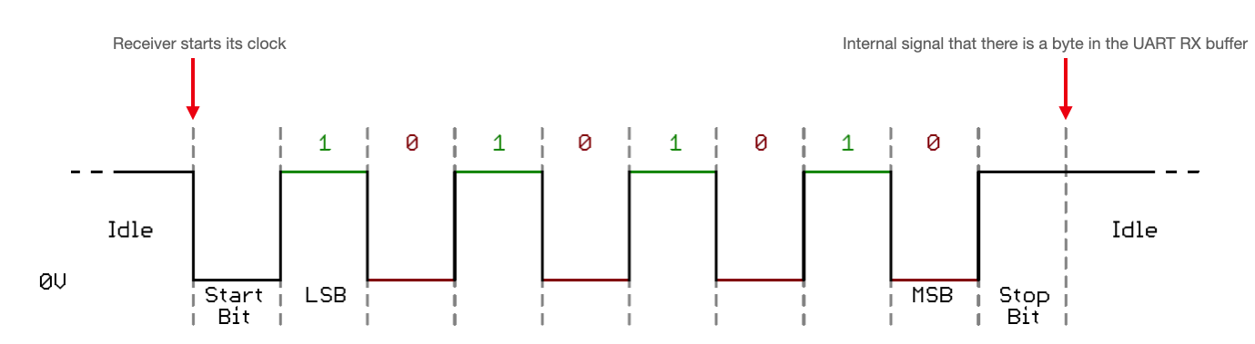
Image source: https://vanhunteradams.com/Protocols/UART/UART.html
I2C
I2C (Inter‑Integrated Circuit) is a synchronous two‑wire bus intended for short‑range, on‑board communication.
I2C topology:
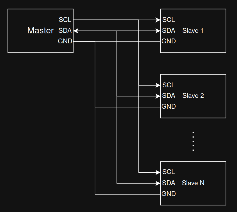
Key characteristics:
- Wires: SDA (data) and SCL (clock). Lines are open‑drain/open‑collector and require pull‑up resistors.
- Roles: Master and slave; multi‑master is supported by the spec but less common in simple designs.
- Addressing: 7‑bit (typical). Devices respond to their address; no separate chip‑select lines.
- Speeds: Standard (100 kHz), Fast (400 kHz), Fast Mode Plus (1 MHz), High‑Speed (3.4 MHz). Effective throughput is lower due to protocol overhead and clock stretching.
- Electrical: Keep bus traces short; choose appropriate pull‑up values based on capacitance and desired rise time.
Because I2C uses only two wires shared by many devices (and GND), it’s ideal for connecting multiple sensors or peripherals at modest speeds.
I2C timing:
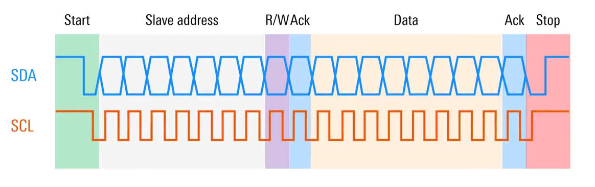
Image source: https://www.youtube.com/watch?v=CAvawEcxoPU
SPI
SPI (Serial Peripheral Interface) is a fast, full‑duplex serial bus commonly used for sensors, displays, and memory devices.
SPI topology:
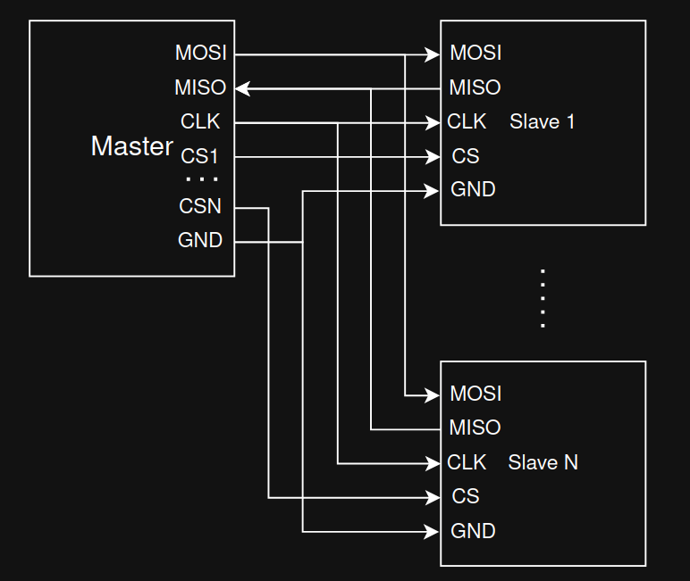
Key characteristics:
- Wires: SCLK (clock), MOSI (master out, slave in), MISO (master in, slave out), and one CS/SS (chip select) per slave.
- Full‑duplex: Data can be transmitted and received simultaneously.
- Modes: Defined by clock polarity (CPOL) and clock phase (CPHA); four modes (0–3). Master and slave must use the same mode and bit order (MSB‑first is common).
- Speed: Often several MHz to tens of MHz depending on hardware and wiring quality.
- Topology: One CS line per device is simplest. Daisy‑chain is possible with some devices but less common.
SPI does not use addresses; the master selects a single slave by asserting its CS line.
SPI timing:
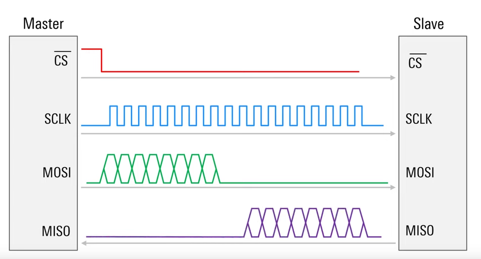
Image source: https://www.youtube.com/watch?v=0nVNwozXsIc
CAN
CAN (Controller Area Network) is a robust, differential multi‑drop bus designed for reliability in noisy environments (originally automotive, now used widely in industry and robotics).
CAN topology:
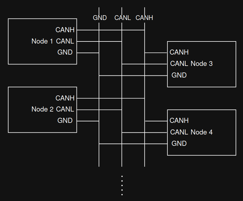
Key characteristics:
- Physical layer: Two wires (CAN‑H, CAN‑L) with 120 Ω terminations at both ends of the main bus. Keep stubs short to reduce reflections.
- Arbitration: Messages have identifiers (11‑bit standard, 29‑bit extended). Non‑destructive arbitration ensures that the highest‑priority (lowest ID) message wins if multiple nodes transmit simultaneously.
- Frames and reliability: Frames contain SOF, arbitration field (ID), control/DLC, data (0–8 bytes for Classical CAN), CRC, ACK, and EOF. Strong error detection, automatic retransmission, and error confinement.
- Bit rates: Classical CAN up to 1 Mbit/s on short buses. CAN‑FD increases data field (up to 64 bytes) and allows higher data‑phase bit rates (e.g., 2–5 Mbit/s) on capable hardware.
Because of its priority‑based arbitration and error handling, CAN is well‑suited for safety‑critical or distributed control systems.
CAN data frame:

Image source: https://en.wikipedia.org/wiki/CAN_bus
When to Use Which
- UART: Point‑to‑point links, simple device logs, GPS modules, Bluetooth modules; low pin count, modest speed.
- I2C: Many low/medium‑speed peripherals on the same PCB, minimal wiring; requires pull‑ups; address management needed.
- SPI: High‑speed peripheral access (displays, flash memory, camera); more pins but excellent throughput and timing control.
- CAN: Robust multi‑drop networking with priorities and error handling across meters of cable; ideal for vehicles and industrial robots.
Resources
- UART overview: https://vanhunteradams.com/Protocols/UART/UART.html
- I2C specification (NXP user manual): https://www.nxp.com/docs/en/user-guide/UM10204.pdf
- SPI basics (Motorola/NXP app notes): https://www.nxp.com/docs/en/application-note/AN2910.pdf
- CAN bus (Wikipedia, overview): https://en.wikipedia.org/wiki/CAN_bus
- CAN‑FD (Bosch spec summary): https://www.bosch-semiconductors.com/ip-modules/can-fd/
Ubuntu Environment
This guide provides step-by-step instructions for setting up the system, installing essential tools, and configuring the environment for ROS2.
sudo apt update
sudo apt upgrade

#swap
sudo fallocate -l 16G /swapfile
sudo chmod 600 /swapfile
sudo mkswap /swapfile
sudo swapon /swapfile
sudo swapon --show


# basic installs
sudo apt install vim git htop cmake build-essential clang net-tools -y openssh-server mc tree

# ROS2
locale  # check for UTF-8
sudo apt update && sudo apt install locales
sudo locale-gen en_US en_US.UTF-8
sudo update-locale LC_ALL=en_US.UTF-8 LANG=en_US.UTF-8
export LANG=en_US.UTF-8
locale  # verify settings

sudo apt install software-properties-common
sudo add-apt-repository universe

sudo apt update && sudo apt install curl -y
sudo curl -sSL https://raw.githubusercontent.com/ros/rosdistro/master/ros.key -o /usr/share/keyrings/ros-archive-keyring.gpg

echo "deb [arch=$(dpkg --print-architecture) signed-by=/usr/share/keyrings/ros-archive-keyring.gpg] http://packages.ros.org/ros2/ubuntu $(. /etc/os-release && echo $UBUNTU_CODENAME) main" | sudo tee /etc/apt/sources.list.d/ros2.list > /dev/null

sudo apt update
sudo apt upgrade
sudo apt install ros-humble-desktop
sudo apt install ros-dev-tools

sudo snap install code --classic
sudo snap install clion --classic
sudo snap install pycharm-community --classic
sudo snap install rustrover --classic

sudo apt update
sudo apt install ros-humble-image-transport-plugins -y