Differential Chassis

The differential drive chassis is one of the most common configurations for mobile robots. It consists of two independently controlled wheels mounted on the same axis and optionally a passive caster wheel for stability.

This tutorial introduces the fundamental concepts of differential drive kinematics and demonstrates how to derive the forward and inverse kinematics equations.

Components of a Differential Drive Chassis

• Two wheels: Independently driven, providing linear and rotational motion.
• Chassis: Holds the wheels, motors, and sensors.
• Center of the robot: Defined as the midpoint between the two wheels.
• Wheel radius (r): Radius of each wheel.
• Wheel separation (L): Distance between the two wheels.

Kinematic Model

Pose (x,y,θ): The robot's position (x,y) and orientation θ in a 2D plane. [m, m, rad]

Linear velocity (v): Forward speed of the robot. [m/s]

Angular velocity (ω): Rate of rotation of the robot. [rad/s]

Conventions:

• Coordinate frame: x points forward, y points to the left (right-handed frame).
• Positive angular velocity ω is counter-clockwise (CCW).
• Wheel linear speeds v_L, v_R are positive when rolling forward.

Wheel Velocities

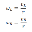
Left wheel angular velocity: ω_L Right wheel angular velocity: ω_R

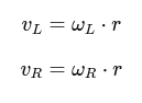
The linear velocities of the wheels are (v_L = r·ω_L, v_R = r·ω_R):

Forward Kinematics

Forward kinematics calculates the robot's linear and angular velocities based on wheel velocities.

Linear and Angular Velocities

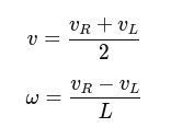
The robot's linear velocity (v) and angular velocity (ω) are:

Turning radius and ICC

• Instantaneous Center of Curvature (ICC) lies at distance R = v/ω from the robot center, to the left for ω > 0 and to the right for ω < 0.
• Special cases:
  • Straight motion: ω = 0 → R = ∞.
  • In-place rotation: v = 0, ω ≠ 0 → R = 0 (wheels spin in opposite directions with equal speed).

Pose Update

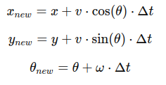
Given the robot's current pose (x,y,θ), the new pose after a small time step dt can be computed as:

Inverse Kinematics

Inverse kinematics computes the wheel velocities required to achieve a desired linear and angular velocity.

Given:

• Desired linear velocity v.
• Desired angular velocity ω.

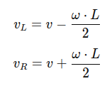
The wheel velocities are:

To compute angular velocities:

Example Code

def forward_kinematics(v_L, v_R, L):
    v = (v_R + v_L) / 2
    omega = (v_R - v_L) / L
    return v, omega

import math

def update_pose(x, y, theta, v, omega, dt):
    x_new = x + v * math.cos(theta) * dt
    y_new = y + v * math.sin(theta) * dt
    theta_new = theta + omega * dt
    # Optional: normalize heading to [-pi, pi)
    if theta_new > math.pi:
        theta_new -= 2 * math.pi
    elif theta_new <= -math.pi:
        theta_new += 2 * math.pi
    return x_new, y_new, theta_new

def inverse_kinematics(v, omega, L):
    v_L = v - (omega * L / 2)
    v_R = v + (omega * L / 2)
    return v_L, v_R

Exercise

Write a program that simulates a differential-drive chassis based on the given input parameters.

Simulation Parameters

• Wheel radius: r = 0.1 m
• Wheel separation: L = 0.15 m
• Time step: dt = 0.01 s

Tasks

• Compute the pose of the robot after moving straight for 5 seconds with v = 1 m/s.
• Simulate a circular motion with v = 1 m/s and ω = 0.5 rad/s.
• Simulate a circular motion with v_L = 1.0 m/s and v_R = 0.5 m/s.
• Optional: If using wheel angular speeds instead, compute v_L = r·ω_L and v_R = r·ω_R first.