PID

This tutorial introduces the concept of PID control and demonstrates how to implement it in a step-by-step manner, suitable for university-level students.

Proportional-Integral-Derivative (PID) control is one of the most widely used control algorithms in engineering and robotics. It is a feedback control mechanism used to maintain a desired setpoint by minimizing error in dynamic systems. PID controllers are found in applications ranging from industrial machinery to autonomous robots.

PID Basics

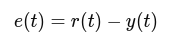
A PID controller continuously calculates an error value e(t), which is the difference between a desired setpoint r(t) and a measured process variable y(t):

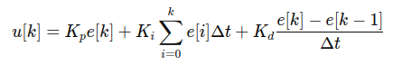
The controller output u(t) is computed as:

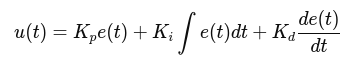
where:

• Kp is Proportional gain.
• Ki is Integral gain.
• Kd is Derivative gain.

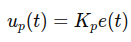
Proportional Control Kp:

Responds to the current error. Larger Kp leads to a faster response but may overshoot.

Integral Control Ki

Responds to the accumulation of past errors. Helps eliminate steady-state error.

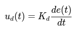
Derivative Control Kd

Responds to the rate of change of the error. Predicts future behavior and reduces overshoot.

PID Implementation

In digital systems, the continuous equation is approximated using discrete time intervals (dt):

Algorithm

• Measure the current system output y[k].
• Calculate the error: e[k] = r[k] − y[k].
• Compute the proportional, integral, and derivative terms.
• Combine the terms to compute u[k].
• Apply u[k] to the system.
• Repeat.

Example Code

class PIDController:

    def __init__(self, kp, ki, kd, setpoint):
        self.kp = kp 
        self.ki = ki  
        self.kd = kd 
        self.setpoint = setpoint

        self.previous_error = 0
        self.integral = 0

    def update(self, measured_value, dt):
        error = self.setpoint - measured_value
        
        # P
        proportional = self.kp * error
        
        # I
        self.integral += error * dt
        integral = self.ki * self.integral
        
        # D
        derivative = self.kd * (error - self.previous_error) / dt
        
        self.previous_error = error
        output = proportional + integral + derivative
        return output

PID Tuning

Manual Tuning

Start with Ki = 0 and Kd = 0. Increase Kp until the system oscillates. Increase Kd to dampen oscillations. Introduce Ki to eliminate steady-state error.

Ziegler-Nichols Method

Set Ki=0 and Kd = 0. Increase Kp until the system oscillates with constant amplitude. Note the critical gain Ku and period Tu. Set parameters as:

• Kp = 0.6 * Ku
• Ki = 2 * Kp / Tu
• Kd = Kp * Tu / 8

Common Problems

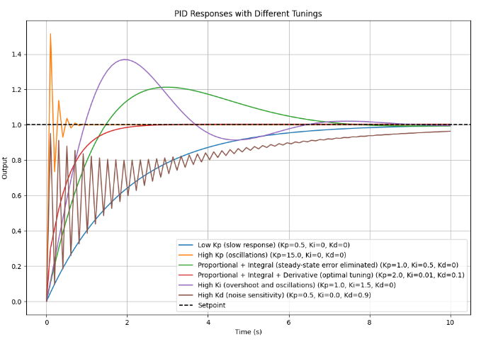
• Low Kp (slow response): The system reacts very slowly, taking a long time to reach the setpoint.
• High Kp (oscillations): The system overshoots and oscillates around the setpoint without damping.
• Proportional + Integral (steady-state error eliminated): The system reaches the setpoint but with overshoot and slower settling time.
• Proportional + Integral + Derivative (optimal tuning): The system reaches the setpoint quickly and without overshoot, showing balanced performance.
• High Ki (overshoot and oscillations): Integral action dominates, causing overshoot and sustained oscillations.
• High Kd (noise sensitivity): The derivative term overly reacts to changes, leading to instability or erratic behavior.